Solving ODE systems and Higher Order ODEs

We first consider a first-order ODE system composed of a set of $N$ simultaneous first-order explicit ODEs:

$$y'_i(t)=f_i(t,\,y_1(t),\cdots,y_N(t))\;\;\;\;\;\;\;\;(i=1,\cdots,N)$$ (109)

The goal is to find the $N$ functions $y_1(t),\cdots,y_N(t)$ that satisfy these $N$ equations based on the $N$ initial conditions $y_i(0)=y_{0i}$ $(i=1,\cdots,N)$. This system can be represented in vector form:

$${\bf y}'(t)=\frac{d}{dt}{\bf y}(t)={\bf f}(t,\,y_1(t),\cdots,y_N(t)) ={\bf f}(t,\,{\bf y}(t)),\;\;\;\;\;\; {\bf y}(0)={\bf y}_0$$ (110)

where

$${\bf y}(t)=\left[\begin{array}{c}y_1(t)\\ \vdots\\ y_N(t)\end{arr... ...{array}{c}f_1(t,\,{\bf y}(t))\\ \vdots\\ f_N(t,\,{\bf y}(t))\end{array}\right]$$ (111)

Consider as an example a special ODE system containing $N$ first-order LCCODEs:

$$\frac{d}{dt}\left[\begin{array}{c}y_1(t)\\ \vdots\\ y_N(t)\end{ar... ...array}\right] +\left[\begin{array}{c}x_1(t)\\ \vdots\\ x_N(t)\end{array}\right]$$ (112)

which can be expressed in matrix form as

$${\bf y}'(t)={\bf Ay}(t)+{\bf x}(t),\;\;\;\; \;\;\;\; {\bf y}'(t)-{\bf Ay}(t)={\bf x}(t)$$ (113)

First, to find the homogeneous solution when ${\bf x}(t)={\bf0}$, we assume ${\bf y}(t)=e^{\lambda t}{\bf v}$ and substitute this into the ODE system to get:

$${\bf y}'(t)=\lambda \,e^{\lambda t}{\bf v}={\bf A} e^{\lambda t}{\bf v}$$ (114)

Dividing both sides by $e^{\lambda t}\ne 0$, we get the eigenequation of ${\bf A}$:

$${\bf Av}=\lambda {\bf v}$$ (115)

where $\lambda$ is an eigenvalue of ${\bf A}$ and ${\bf v}$ is the corresponding eigenvector. In general, there are $N$ eigenvalues $\{\lambda_1,\cdots,\lambda_N\}$ and $N$ corresponding eigenvectors $\{{\bf v}_1,\cdots,{\bf v}_N\}$ for an $N$ by $N$ matrix ${\bf A}$, and the homogeneous solution is a linear combination of all $N$ such solutions:

$${\bf y}_h(t)=\sum_{i=1}^N c_i e^{\lambda_it}{\bf v}_i =[{\bf v}_1... ...array}{c} c_1\\ \vdots\\ c_N\end{array}\right] ={\bf V}e^{{\bf\Lambda}t}{\bf c}$$ (116)

where $e^{{\bf\Lambda}t}$ is a matrix exponential function, which is generally defined based on the Taylor expansion of an exponential function:

$$e^{\bf A}={\bf I}+{\bf A}+\frac{1}{2!}{\bf A}^2 +\frac{1}{3!}{\bf A}^3+\cdots$$ (117)

Specially when ${\bf A}={\bf\Lambda t}$ is a diagonal matrix, we have

$$e^{\bf\Lambda t} ={\bf I}+{\bf\Lambda t}+\frac{1}{2!}{\bf\Lambda}... ...&&e^{\lambda_Nt} \end{array}\right] =diag[e^{\lambda_1t},\cdots,e^{\lambda_Nt}]$$ (118)

The $N$ coefficients in ${\bf c}=[c_1,\cdots,c_N]^T$ can be found based on the $N$ given initial conditions ${\bf y}(0)={\bf y}_0$:

$${\bf y}(0)={\bf y}(t)\bigg\vert _{t=0} ={\bf V}e^{{\bf\Lambda}t}{\bf c}\bigg\vert _{t=0}={\bf Vc}={\bf y}_0$$ (119)

Solving for ${\bf c}$ we get ${\bf c}={\bf V}^{-1}{\bf y}_0$. Substituting this back to the general solution we get:

$${\bf y}_h(t)={\bf V}e^{{\bf\Lambda}t}{\bf c} ={\bf V}e^{{\bf\Lambda}t}{\bf V}^{-1}{\bf y}_0$$ (120)

But as the eigenvalue and eigenvector matrices ${\bf\Lambda}$ and ${\bf V}$ of ${\bf A}$ satisfy ${\bf AV}={\bf V\Lambda}$ or ${\bf A}={\bf V\Lambda V}^{-1}$, we have

$${\bf V}e^{\bf\Lambda}{\bf V}^{-1} = {\bf V}\left({\bf I}+{\bf\Lambda}+\frac{1}{2!}{\bf\Lambda}^2+\cdo... ...V\Lambda V}^{-1}+\frac{1}{2!} {\bf V\Lambda V}^{-1}{\bf V\Lambda V}^{-1}+\cdots$$

$$= {\bf I}+{\bf A}+\frac{1}{2!}{\bf A}^2+\cdots=e^{\bf A}$$ (121)

Therefore the homogeneous solution can be written as

$${\bf y}_h(t)={\bf V}e^{{\bf\Lambda}t}{\bf V}^{-1}{\bf y}_0=e^{{\bf A}t}{\bf y}_0$$ (122)

Next, in the non-homogeneous case when ${\bf x}\ne {\bf0}$, the complete solution of the first-order LCCODE system can again be found analytically. We first multiply $e^{-{\bf A}t}$ on both sides of the ODE ${\bf y}'(t)-{\bf Ay}(t)={\bf x}(t)$ and get

$$e^{-{\bf A}t} {\bf y}'(t)-e^{-{\bf A}t}{\bf Ay}(t) =\frac{d}{dt}\left[ e^{-{\bf A}t} {\bf y}(t) \right] =e^{-{\bf A}t}{\bf x}(t)$$ (123)

Integrating both sides we get

$$\int_0^t\frac{d}{d\tau}\left[ e^{-{\bf A}\tau} {\bf y}(\tau)\righ... ...-{\bf A}t}{\bf y}(t)-{\bf y}(0) =\int_0^t e^{-{\bf A}\tau}{\bf x}(\tau) \;d\tau$$ (124)

Multiplying $e^{{\bf A}t}$ on both side and rearranging we get

$${\bf y}(t)=e^{{\bf A}t}{\bf y}(0)+e^{{\bf A}t}\int_0^t e^{-{\bf A... ...+\int_0^t e^{{\bf A}(t-\tau)}{\bf x}(\tau) \;d\tau\ ={\bf y}_h(t)+{\bf y}_p(t)$$ (125)

where ${\bf y}_h(t)=e^{{\bf A}t}{\bf y}(0)$ is the homogeneous solution same as that found previously, and ${\bf y}_p(t)$ is the particular solutions, the system response to the input ${\bf x}(t)$. Specially when ${\bf x}(t)={\bf\delta}(t)$ is an impulse function, the system response is the impulse response of the system:

$${\bf y}_p(t)=\int_0^t e^{{\bf A}(t-\tau)}{\bf\delta}(\tau) \;d\tau=e^{{\bf A}t}$$ (126)

i.e., the particular solution is the convolution of the impulse response and the input:

$${\bf y}_p(t)=\int_0^t e^{{\bf A}(t-\tau)}{\bf x}(\tau) \;d\tau\ =e^{{\bf A}t}\,*\,{\bf x}(t)$$ (127)

The stability of the solution found above depends on the eigenvalues $\{\lambda_1,\cdots,\lambda_N\}$. If they all have negative real part, then the solution ${\bf y}(t)$ is stable at it will always converge to ${\bf0}$. However, if one or more eigenvalues have positive real parts while others have negative parts, a saddle point, then the solution is unstable as it will approach $\pm\infty$ as $t\longrightarrow\infty$.

We next consider an Nth-order scalar ODE in the following explicit form

$$\frac{d^N}{dt^N}y(t)=y^{(N)}(t)=f(t,\,y'(t),\cdots,y^{(N-1)}(t))$$ (128)

The goal is to find $y(t)$ satisfying this equation and some given initial condition $y(0)=y_0$. To solve this DE, we can convert it into a first-order ODE system containing $N$ first-order ODEs. Specifically, we define $y_i(t)=y^{(i-1)}(t)$ ( $i=1,\cdots,N$) and represent these $N$ functions in vector form:

$${\bf y}(t)=\left[\begin{array}{c}y_1(t)\\ y_2(t)\\ y_3(t)\\ \vdot... ...t)\\ y'_1(t)\\ y'_2(t)\\ \vdots\\ y'_{N-2}(t)\\ y'_{N-1}(t) \end{array} \right]$$ (129)

so that the Nth-order ODE can be convered into $N$ first-order ODEs:

$$\frac{d}{dt}{\bf y}(t)={\bf y}'(t) =\left[\begin{array}{c}y'_1(t)... ... \vdots\\ y_N(t)\\ f(t,\,{\bf y}(t))\end{array}\right] ={\bf f}(t,\,{\bf y}(t))$$ (130)

The last equation is the original Nth-order ODE:

$$y'_N(t)=y^{(N)}(t)=\frac{d^N}{dt^N}y(t) = f(t,y(t),y'(t),y''(t),\cdots,y^{(N-1)}(t))$$

$$= f(t,\,y_1(t),y_2(t),y_3(t),\cdots,y_N(t))=f(t,\,{\bf y}(t))$$ (131)

Reconsider as an example the second order LCCODE in canonical form:

$$y''(t)+2\zeta\omega_n y(t)+\omega_n^2 y(t)=x(t)$$ (132)

Here we first convert it into a first order equation system by introducing $y_1=y,\;y_2=y'$:

$$\left\{ \begin{array}{l} y'_1=y'=y_2 \\ y'_2=y''=-2\zeta\omega_n y'-\omega_n^2y+x(t) =-2\zeta\omega_ny_2-\omega_n^2y_1+x(t) \end{array}\right.$$ (133)

or in matrix form

$${\bf y}'(t)=\left[\begin{array}{c}y_1'(t)\\ y_2'(t)\end{array}\ri... ...ray}\right] +\left[\begin{array}{c}0\\ x(t)\end{array}\right] ={\bf Ay}+{\bf x}$$ (134)

To solve this system, we first solve the eigenvalue problem of the coefficient matrix ${\bf A}$. Solving its characteristic equation:

$$\det(\lambda{\bf I}-{\bf A}) =\det\left[\begin{array}{cc}\lambda ... ...2\zeta\omega_n \end{array}\right] =\lambda^2+2\zeta\omega_n\lambda+\omega_n^2=0$$ (135)

we get the eigenvalues of ${\bf A}$ the two eigenvalues and the eigenvalue matrix:

$$\lambda_{1,2}=\left(-\zeta\pm\sqrt{\zeta^2-1}\right)\omega_n =\le... ...\Lambda}=\left[\begin{array}{cc}\lambda_1 & 0\\ 0 & \lambda_2\end{array}\right]$$ (136)

Note that

$$\lambda_1\lambda_2=\omega_n^2,\;\;\;\;\;\;\;\;\;\; \lambda_2-\lambda_1=2\omega_n\sqrt{\zeta^2-1}$$ (137)

The corresponding eigenvectors can be found by solving the following homogeneous equation:

$$(\lambda_i{\bf I}-{\bf A}) {\bf v}_i =\left[\begin{array}{cc}\lam... ...rray}\right] =\left[\begin{array}{c}0\\ 0\end{array}\right],\;\;\;\;\;\;(i=1,2)$$ (138)

to get ${\bf v}_1=[1,\;\lambda_1]^T$ and ${\bf v}_2=[1,\;\lambda_2]^T$, and

$${\bf V}=\left[\begin{array}{cc}1 & 1\\ \lambda_1 & \lambda_2\end{... ...bda_1} \left[\begin{array}{cc}\lambda_2 & -1\\ -\lambda_1 & 1\end{array}\right]$$ (139)

and we can verify thatat ${\bf AV}={\bf V\Lambda}$. The general form of the homogeneous solution is

$${\bf y}=\left[\begin{array}{c}y_1\\ y_2\end{array}\right] =c_1 {\... ...bda_1t} +c_2\left[\begin{array}{c}1\\ \lambda_2\end{array}\right]e^{\lambda_2t}$$ (140)

i.e.,

$$\left\{ \begin{tabular}{l} $y_1(t)=y(t)=c_1e^{\lambda_1t}+c_2e^{\... ...(t)=c_1\lambda_1e^{\lambda_1t}+c_2\lambda_2e^{\lambda_2t}$ \end{tabular}\right.$$ (141)

• Homogeneous case:

  We have $x(t)=0$ and assume $y_1(0)=y(0)=y_0$ and $y_2(0)=y'(0)=0$. Evaluating the general solution above at $t=0$, we get:

  $$\left\{ \begin{tabular}{l} $y_1(0)=y(0)=c_1+c_2=y_0$\\ $y_2(0)=y'_1(0)=c_1\lambda_1+c_2\lambda_2=0$ \end{tabular}\right.$$ (142)

  Solving this we get

  $$C_1=\frac{\lambda_2}{\lambda_2-\lambda_1}y_0,\;\;\;\;\;\;\;\; C_2=\frac{\lambda_1}{\lambda_1-\lambda_2}y_0$$ (143)

  Substituting into $y_1(t)=y(t)$ above, we get:

  $$y(t)=y_1(t)=\frac{y_0}{\lambda_2-\lambda_1}(\lambda_2e^{\lambda_1t}-\lambda_1e^{\lambda_2t})$$ (144)

  Alternatively, we can also get
  

  $${\bf y}(t) = e^{{\bf A}t}{\bf y}(0)={\bf V}e^{{\bf\Lambda}t}{\bf V}^{-1}{\bf y... ...\lambda_1&1\end{array}\right] \left[\begin{array}{c} y_0 \\ 0\end{array}\right]$$

  $$= \frac{1}{\lambda_2-\lambda_1} \left[\begin{array}{cc} \lambda_2e^... ...\lambda_1t}\end{array}\right] \left[\begin{array}{c} y_0 \\ 0\end{array}\right]$$

  $$= \frac{y_0}{\lambda_2-\lambda_1} \left[\begin{array}{c} \lambda_2e... ...bda_2t}\\ \lambda_1\lambda_2(e^{\lambda_1t}-e^{\lambda_2t}) \end{array}\right]$$

  
  we get the same result as shown above:

  $$y(t)=y_1(t)=\frac{y_0}{\lambda_2-\lambda_1}(\lambda_2e^{\lambda_1t}-\lambda_1e^{\lambda_2t})$$ (145)

• Nonhomogeneous case:

  We assume $x(t)=u(t)$ and zero initial conditions $y_1(0)=y_2(0)=0$, i.e., ${\bf x}=[0,\;1]^T$ and ${\bf y}={\bf0}$, and get:

  $${\bf y}(t)=e^{{\bf A}t}{\bf y}(0)+e^{{\bf A}t}\int_0^t e^{-{\bf A}\tau}{\bf x}(\tau)d\tau =e^{{\bf A}t}\int_0^t e^{-{\bf A}\tau} d\tau \;[0,\;1]^T$$ (146)

  and

  $$y_h(t)=y_1(t)=[1,\;0]\;{\bf y}(t)=[1,\;0]\; e^{{\bf A}t}\int_0^t e^{-{\bf A}\tau} d\tau\; [0,\;1]^T$$ (147)

  where

  $$\int_0^t e^{-{\bf A}\tau} d\tau=-{\bf A}^{-1} e^{-{\bf A}\tau}\bigg\vert _0^t ={\bf A}^{-1}( {\bf I}-e^{-{\bf A}t} )$$ (148)

  Substituting

  $${\bf A}^{-1}=({\bf V\Lambda V}^{-1})^{-1}={\bf V\Lambda}^{-1}{\bf... ...t}{\bf V}^{-1},\;\;\;\;\;\; e^{-{\bf A}t}={\bf V}e^{-{\bf\Lambda}t}{\bf V}^{-1}$$ (149)

  into the function, we get
  

  $$y(t) = [1,\;0]\;\left(e^{{\bf A}t}\int_0^t e^{-{\bf A}\tau} d\tau\right)... ...1}\right) \left({\bf I}-{\bf V}e^{-{\bf\Lambda}t}{\bf V}^{-1}\right)\;[0,\;1]^T$$

  $$= [1,\;0]\;{\bf V}e^{{\bf\Lambda}t} {\bf\Lambda}^{-1}{\bf V}^{-1} -... ...Lambda}t}{\bf\Lambda}^{-1}({\bf I}-e^{-{\bf\Lambda}t} ){\bf V}^{-1} \;[0,\;1]^T$$

  $$= [1,\;0]\;\left[\begin{array}{cc}1&1\\ \lambda_1&\lambda_2\end{arr... ...\\ -\lambda_1&1\end{array}\right] \left[\begin{array}{c}0\\ 1\end{array}\right]$$

  $$= \left[e^{\lambda_1t},\;e^{\lambda_2t}\right] \left[\begin{array}{... ...ac{\lambda_2e^{\lambda_1t}-\lambda_1e^{\lambda_2t}}{\lambda_2-\lambda_1}\right)$$

  
  

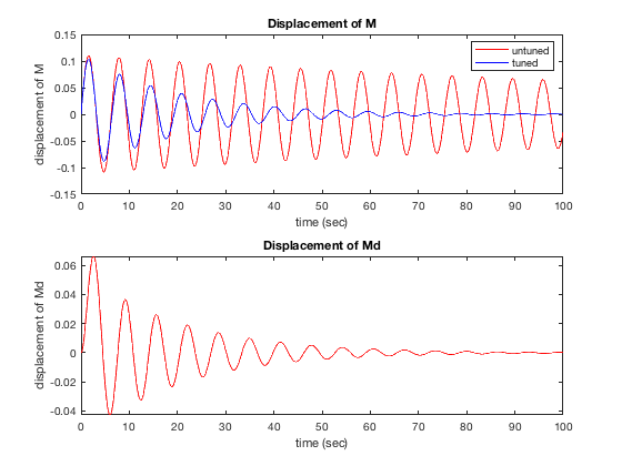
Example 2: A tuned mass-damper-spring system shown below is described by the following ODEs:

$$\left\{\begin{array}{l} My''=-Ky-Cy'-K_d(y-y_d)-C_d(y'-y_d')+f(t)\\ M_d y_d''=K_d(y-y_d)+C_d(y'-y_d')\end{array}\right.$$ (150)

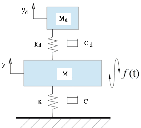
This 2nd-order ODE system can be converted into a 1st-order ODE system by introducing $v=y'$ and $v_d=y_d'$:

$$\left\{\begin{array}{l} y'=v\\ v'=[-Ky-Cy'-K_d(y-y_d)-C_d(y'-y_d')+f]/M\\ y_d'=v_d\\ v_d'=[K_d(y-y_d)+C_d(y'-y_d')/M_d\end{array}\right.$$ (151)

or in matrix form

$${\bf y}'= \left[\begin{array}{c}y'\\ v'\\ y_d'\\ v_d'\end{array}\... ...eft[\begin{array}{c}0\\ \frac{f}{M}\\ 0\\ 0\end{array}\right] ={\bf Ay}+{\bf x}$$ (152)

Specifically, if we assume $f(t)=\delta(t)$ (modeling an earthquake) i.e., ${\bf x}=[0,\;\delta(t)/M,\;0,\;0]^T$, and all zero initial condition ${\bf y}(0)={\bf0}$, then we get:

$${\bf y}=\int_0^t e^{{\bf A}(t-\tau)}{\bf x}(\tau)d\tau$$ (153)

and $y(t)$ as the first component of ${\bf y}$ is

$$y(t)={\bf y}(1)={\bf v}_1^Te^{{\bf\Lambda}t}{\bf u}_2$$ (154)

where ${\bf v}_1^T$ and ${\bf u}_2$ are respectively the first row of ${\bf V}$ and the second column of ${\bf V}^{-1}$.