Here we consider specifically solving Nth order LCCODEs with
 ,
,  , and
, and  .
.
Solving first-order LCCODE:
 |
(37) |
with an initial condition
 .
.
We first find the homogeneous solution, denoted by  ,
that satisfies
,
that satisfies
 due to the non-zero initial
condition
due to the non-zero initial
condition  , and then find the particular solution,
denoted by
, and then find the particular solution,
denoted by  , that satisfies
 . Due
to the linearity of the equation, the sum
. Due
to the linearity of the equation, the sum
 of
the homogeneous and a particular solution is also a solution, called
the complete solution.
of
the homogeneous and a particular solution is also a solution, called
the complete solution.
To find the homogeneous solution, we assume
 , and
substitute it into the ODE to get
, and
substitute it into the ODE to get
 |
(38) |
Dividing both sides by
 , we get
  , i.e,
 . The coefficient
  is determined by the
initial condition. Evaluating at
is determined by the
initial condition. Evaluating at  we get
 |
(39) |
and the homogeneous solution is
 |
(40) |
To find the complete solution of the nonhomogeneous ODE with
 , we first multiply both sides of the ODE by
  :
:
![$\displaystyle e^{at} \left[ y'(t)+a\,y(t) \right]
=e^{at} y'(t)+a e^{at}y(t)=e^{at} x(t)$](img107.svg) |
(41) |
and rewrite it as
![$\displaystyle \frac{d}{dt} \left[ e^{at}y(t) \right]=e^{at}x(t)$](img108.svg) |
(42) |
and then integrate both sides to get
 |
(43) |
Multiplying both sides by  and rearranging, we get the
expression for
and rearranging, we get the
expression for 
![$\displaystyle y(t)=e^{-at}\left[ y(0)+\int_0^t e^{a\tau}x(\tau) d\tau \right]
=e^{-at}y_0+\int_0^t e^{-a(t-\tau)}x(\tau) d\tau
=y_h(t)+y_p(t)$](img111.svg) |
(44) |
where
 is the homogeneous solution same as
that found above, and is the particular solution:
is the homogeneous solution same as
that found above, and is the particular solution:
 |
(45) |
In particular, if the input
 is a unit impulse
(Derac dilta function), we get the impulse response
is a unit impulse
(Derac dilta function), we get the impulse response
 . We therefore see that in general, the
particular solution is the convolution of the impulse response
. We therefore see that in general, the
particular solution is the convolution of the impulse response
 and the input
  .
.
Alternatively, we can also solve the first order LCCODE by the
method of Laplace transform. Specifically, we take Laplace
transform on both sides of the equation to get
![$\displaystyle {\cal L}\left[ \;y'(t)+ay(t)\;\right]
=sY(s)-y(0)={\cal L}\left[ \;x(t)\;\right]=X(s)$](img116.svg) |
(46) |
Solving for  we get the solution in s-domain:
 |
(47) |
Taking inverse transform we get the solution in time domain:
![$\displaystyle y(t)={\cal L}^{-1} \left[\frac{y_0}{s+a}\right]
+{\cal L}^{-1}\left[ \frac{X(s)}{s+a}\right]
=y_0e^{-at}+x(t)\;*\;e^{-at}$](img118.svg) |
(48) |
where
 is the homogeneous solution, and
 as the convolution of the input
and the impulse response of the system is
the particular solution.
as the convolution of the input
and the impulse response of the system is
the particular solution.
- Constant input:
Taking the unilateral Laplace transform of the equation
 we get
![$\displaystyle {\cal L}\left[y'(t)+a y(t)\right]=sY(s)-y_0+aY(s)
={\cal L}\left[u(t)\right]=\frac{1}{s}$](img122.svg) |
(49) |
Solving for , we further get
 |
(50) |
Taking the inverse Laplace trannsform we get the solution in
time domain:
 |
(51) |
- Sinusoidal input:
To solve the ODE with a sinusoidal input
 , we first consider a
complex exponontial input
, we first consider a
complex exponontial input
 |
(52) |
Taking the Laplace transform on both sides we get
![$\displaystyle {\cal L}\left[y'(t)+a y(t)\right]=s Y(s)-y_0+a Y(s)
={\cal L}\left[e^{j\omega t}u(t)\right]=\frac{1}{s-j\omega}$](img127.svg) |
(53) |
Solving for , we get
 |
(54) |
Taking the inverse Laplace trannsform we get the solution
in time domain:
where
 . Taking the real part we get the
solution:
. Taking the real part we get the
solution:
Solving second order LCCODE:
 |
(55) |
We first find the homogeneous solution by assuming  . We
assume
. We
assume
 and substitute it with its derivatives
 into the DE and get
 |
(56) |
Dividing both sides by
 , we get an algebraic equation
 |
(57) |
solving which we get its two roots:
 |
(58) |
where
 |
(59) |
and
 |
(60) |
Note that
 |
(61) |
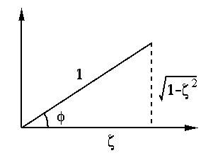
where  is the damped natural frequency defined as:
 |
(62) |
and
 |
(63) |
These two roots  are either two real numbers or a pair
complex conjugate numbers, depending on whether its discriminant
is greater and smaller then 0:
are either two real numbers or a pair
complex conjugate numbers, depending on whether its discriminant
is greater and smaller then 0:
 |
(64) |
As
 for all physical systems,
 for all cases.
For a constant  and a variable
  that changes
from
that changes
from  to
to  , the two roots
  (red) and
  (blue) can be represented as the root locus on the complex plane.
Given the two roots and , we get the homogeneous
solution as the linear combination of the two solutions  and
and  :
:
 |
(65) |
where the two coefficients  and
and  can be found based on
the two initial conditions
can be found based on
the two initial conditions  and
and
 :
:
Solving these we get
 |
(66) |
and the homogeneous solution becomes:
![$\displaystyle y_h(t)=y_0 \left[ \frac{s_2 e^{s_1t}}{s_2-s_1}-\frac{s_1 e^{s_2t}}{s_2-s_1} \right]
=\frac{y_0}{s_2-s_1} (s_2 e^{s_1t}-s_1 e^{s_2t})$](img169.svg) |
(67) |
The solution takes different forms depending on the value of the damping
coefficient .
- Over-damped system (
 )
)
This is a sum of two exponentially decaying terms, without any overshoot
or oscillation. Note that when ,  .
.
- Critically damped system (
 )
)
Now we have
 |
(68) |
and the homogeneous solution takes following form:
Applying the initial conditions to this response we get
Solving this we get
 |
(69) |
and the response is
![$\displaystyle y_h(t)=C_1 e^{st}+C_2 t e^{st}=y_0\left[ e^{-\omega_nt}+\omega_n t e^{-\omega_nt}\right]$](img183.svg) |
(70) |
Again, there is no overshoot or oscillation.
- Under-damped system (
 )
)
 and and |
(71) |
The response is
- Undamped system (
 )
)
 |
(72) |
![$\displaystyle y_h(t)=y_0 \left[ \frac{s_2 e^{s_1t}}{s_2-s_1}+\frac{s_1 e^{s_2t}...
...ght]
=y_0\left(\frac{e^{j\omega_n}+e^{-j\omega_n}}{2}\right)=y_0\cos(\omega_nt)$](img192.svg) |
(73) |
This result can also be obtained from the previous case:
 |
(74) |
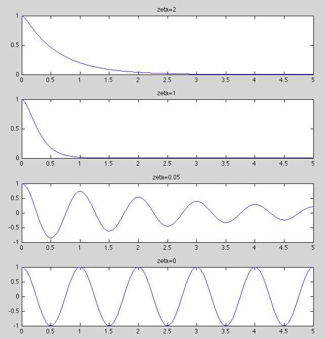
The homogeneous responses of these four cases are plotted below. Note that in all cases,
and
 .
.
We next consider the complete solution of the equation
|
(75) |
with a unit step  input and zero initial conditions
 . As the input is a constant for
  , we can
assume the solution is a constant
, we can
assume the solution is a constant  with zero derivatives
 . Substituting these into the equation, we get
the particular solution (also called the steady state solution:
. Substituting these into the equation, we get
the particular solution (also called the steady state solution:
 |
(76) |
The complete response can now be obtained as the sum of the
homogeneous solution (same as that obtained previously) due
to the non-zero initial condition and the particular solution
due to the non-zero input:
 |
(77) |
The two coefficients and can be obtained based on
the two initial conditions, here assumed to be zero:
Solving these equations we get:
 |
(78) |
Now the complete solution becomes:
![$\displaystyle y(t)=\frac{1}{\omega_n^2}\left[1-\left(\frac{s_2e^{s_1t}}{s_2-s_1...
...ht]
=\frac{1}{\omega_n^2}\left[1-\frac{s_2e^{s_1t}-s_1e^{s_1t}}{s_2-s_1}\right]$](img205.svg) |
(79) |
The two roots and take different forms depending on
whether the discriminant
 is greater
or smaller than 0, i.e., whether is greater or smaller then 1.
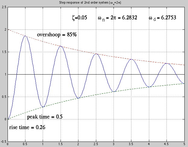
Here we only consider the case when
is greater
or smaller than 0, i.e., whether is greater or smaller then 1.
Here we only consider the case when
 , i.e.,
  ,
for an under-damped second order system. The two roots are
,
for an under-damped second order system. The two roots are
 and and |
(80) |
where is the damped natural frequency:
|
(81) |
Finally the complete solution of the non-homogeneous DE is:
where
 same as that given
above. In particular, if , we have
same as that given
above. In particular, if , we have
![$\displaystyle y(t)=\frac{1}{\omega_n^2}\left[1-\sin(\omega_n t+\pi/2)\right]
=\frac{1}{\omega_n^2}\left[1-\cos(\omega_n t)\right]$](img217.svg) |
(82) |
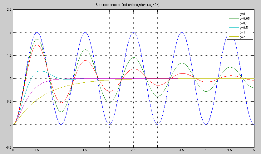
The plots below shows an example with
 . Note
the critical damped case when . An overshoot will occur
for any
. Note
the critical damped case when . An overshoot will occur
for any  .
.
The step response is plotted below. Note that  and
.
and
.
Alternatively, we can also solve the second order LCCODE by the
method of Laplace transform. Specifically, we take Laplace
transform on both sides of the equation to get
 |
(83) |
Dividing both sides by
 and rearranging, we get
 |
(84) |
- Homogeneous case:
If we assume and  , then the above becomes
 |
(85) |
i.e.,
 |
(86) |
Solving for  and
and  we get
 |
(87) |
and
 |
(88) |
- Impulse response:
If we assume
with
![$X(s)={\cal L}[ \delta(t) ]=1$](img76.svg) and zero initial condition
and zero initial condition
 , then the transfer function
is
, then the transfer function
is
 |
(89) |
and the impulse response function is
![$\displaystyle h(t)={\cal L}^{-1}[H(s)]=\frac{1}{s_2-s_1}
{\cal L}^{-1}\left( \f...
...-s_2}-\frac{1}{s-s_1}\right)
=\frac{1}{s_2-s_1}\left( e^{s_2t}-e^{s_1t} \right)$](img233.svg) |
(90) |
Alternatively, we can also find  as
as
Substituting in
 , we further get
- Nonhomogeneous case:
If we assume with
![$X(s)={\cal L}[ u(t) ]=1/s$](img240.svg) and zero initial condition
, then we have
and zero initial condition
, then we have
i.e.,
 |
(94) |
Solving for , and  we get
 |
(95) |
and
 |
(96) |
As shown above, when , we have
![$\displaystyle y(t)=\frac{1}{\omega_n^2}\left[1-\frac{e^{-\zeta\omega_nt}}{\sqrt{1-\zeta^2}}
\sin(\omega_dt+\phi) \right]$](img248.svg) |
(97) |
Alternatively, the same step response can also be found as the convolution
of the impulse response and the input :
where we have used the facts that
 and
and
 , and the integral
![$\displaystyle \int e^{at}\sin(bt)\;dt=\frac{e^{at}}{a^2+b^2}\left[ a\sin(bt)-b\cos(bt)\right]$](img256.svg) |
(99) |
Solving third order LCCODE:
 |
(100) |
with initial conditions
 .
Here we only consider the Homogeneous case.
Let
.
Here we only consider the Homogeneous case.
Let
 be the three roots of the characteristic
equation so that
be the three roots of the characteristic
equation so that
i.e,
 ,
,
 and
and
 .
We let
.
We let
 , and find the
coefficients
, and find the
coefficients
![${\bf c}=[c_1,\;c_2,\;c_3]^T$](img266.svg) by solving the equation
by solving the equation
![$\displaystyle {\bf Sc}=\left[\begin{array}{ccc}1 & 1 & 1\\ s_1 & s_2 & s_3\\
s...
...ray}\right]
=\left[\begin{array}{c}y_0\\ y'_0\\ y''_0\end{array}\right]={\bf y}$](img267.svg) |
(102) |
to get
 , where
![$\displaystyle {\bf S}^{-1}=\left[\begin{array}{ccc}
1 & 1 & 1\\ s_1 & s_2 & s_3...
... s_1s_3 & -(s_1+s_3) & 1\\ s_1s_2 & -(s_1+s_2) & 1
\end{array}\right]
={\bf DR}$](img269.svg) |
(103) |
Alternatively, we can use the method of Laplace transform to get
Equating the coefficients for  and constant terms of the
numerators, we get
and constant terms of the
numerators, we get
![$\displaystyle \left[\begin{array}{ccc}
s_2s_3 & s_1s_3 & s_1s_2\\ -(s_2+s_3) & ...
...
\end{array}\right]
\left[\begin{array}{c} y_0\\ y'_0\\ y''_0\end{array}\right]$](img274.svg) |
(105) |
which can be written as
 i.e., i.e., |
(106) |
But we also note the following identity:
![$\displaystyle {\bf AS}=\left[\begin{array}{ccc} a_1 & a_2 & 1\\ a_2 & 1 & 0\\ 1...
...s_1s_2\\
-(s_2+s_3)&-(s_1+s_3)&-(s_1+s_2)\\ 1&1&1\end{array}\right]
={\bf R}^T$](img277.svg) |
(107) |
i.e.,
 . Substituting this
into the expression for
. Substituting this
into the expression for  we get the same coefficients
found previously:
we get the same coefficients
found previously:
 |
(108) |


![$\displaystyle {\cal L}^{-1} Y(s)=\frac{1}{j\omega+a}\left[ {\cal L}^{-1}
\left(...
...}\left(\frac{1}{s+a}\right)\right]
+{\cal L}^{-1}\left( \frac{y_0}{s+1} \right)$](img129.svg)


![$\displaystyle \frac{1}{\sqrt{\omega^2+a^2}}\cos(\omega t-\phi)
+\left[y_0 -\frac{1}{\sqrt{\omega^2+a^2}}\cos(-\phi)\right] e^{-at}$](img133.svg)


![$\displaystyle y_0 \left[ \frac{s_2 e^{s_1t}}{s_2-s_1}+\frac{s_1 e^{s_2t}}{s_1-s_2} \right]$](img172.svg)
![$\displaystyle y_0\left[\frac{-\zeta+\sqrt{\zeta^2-1}}{2\sqrt{\zeta^2-1}}e^{(-\z...
...qrt{\zeta^2-1}}{2\sqrt{\zeta^2-1}}e^{(-\zeta+\sqrt{\zeta^2-1})\omega_nt}\right]$](img173.svg)


![$\displaystyle \frac{d}{dt}[C_1 e^{st}+C_2 t e^{st}]=C_1se^{st}+C_2(e^{st}+ste^{st})$](img179.svg)


![$\displaystyle y_0 \left[ \frac{s_2 e^{s_1t}}{s_2-s_1}-\frac{s_1 e^{s_2t}}{s_2-s_1} \right]$](img187.svg)
![$\displaystyle y_0\left[ \frac{(-\zeta-j\sqrt{1-\zeta^2})\omega_n}{-2j\omega_n\s...
...)\omega_n}{-2j\omega_n\sqrt{1-\zeta^2}} e^{(-\zeta\omega_n-j\omega_d)t} \right]$](img188.svg)


![$\displaystyle \frac{1}{\omega_n^2}\left[1-\left(\frac{s_2}{s_2-s_1}e^{s_1t}-\frac{s_1}{s_2-s_1}e^{s_2t}\right)\right]$](img211.svg)
![$\displaystyle \frac{1}{\omega_n^2}\left[ 1-
\left(\frac{\zeta+j\sqrt{1-\zeta^2}...
...1-\zeta^2}}{2j\sqrt{1-\zeta^2}} e^{(-\zeta\omega_n-j\omega_d)t} \right) \right]$](img212.svg)
![$\displaystyle \frac{1}{\omega_n^2}\left[ 1-\frac{e^{-\zeta\omega_nt}}{\sqrt{1-\...
...j\omega_dt}
-\frac{\zeta-j\sqrt{1-\zeta^2}}{2j} e^{-j\omega_dt} \right) \right]$](img213.svg)
![$\displaystyle \frac{1}{\omega_n^2}\left[ 1-\frac{e^{-\zeta\omega_nt}}{\sqrt{1-\...
...rac{ e^{j\phi} e^{ j\omega_dt}-e^{-j\phi} e^{-j\omega_dt} }{2j} \right) \right]$](img214.svg)
![$\displaystyle \frac{1}{\omega_n^2}\left[1-\frac{e^{-\zeta\omega_nt}}{\sqrt{1-\zeta^2}}
\sin(\omega_dt+\phi) \right]$](img215.svg)


![$\displaystyle \frac{1}{\omega_n\sqrt{1-\zeta^2}}
\left[\frac{e^{-\zeta\omega_n\...
...(-\zeta\omega_n\sin(\omega_d\tau)-\omega_d\cos(\omega_d\tau)\right)
\right]_0^t$](img250.svg)
![$\displaystyle \frac{1}{\sqrt{1-\zeta^2}} \left[
\frac{e^{-\zeta\omega_n\tau}}{(...
...t(-\zeta\sin(\omega_d\tau)-\sqrt{1-\zeta^2}\cos(\omega_d\tau)\right)\right]_0^t$](img251.svg)

![$\displaystyle \frac{1}{\omega_n^2\sqrt{1-\zeta^2}}\left[ \sin\phi-e^{-\zeta\omega_nt}\sin(\omega_dt+\phi)\right]$](img253.svg)


