Stiffness and stability

As we see in the previous example, due to the change of the system parameters, the problem may become difficult to solve, in the sense that significantly reduced step size and thereby much increased computing time will be needed for the numerical solution to remain bounded. Such problems are said to be stiff, which is hard to be strictly defined mathematically. One way to measure the stiffness of a given problem is the stiffness ratio defined as $Re(s_{max})/Re(s_{min})$, where $\lambda_{max}$ and $\lambda_{min}$ are respectively the eigenvalues of the coefficient matrix ${\bf A}$ with most negative and least negative real part, assuming all eigenvalues have negative real parts. In the example above, the stiffness ratios corresponding to the four sets of parameters are 1, 10, 100, and 1000, i.e., the problem becomes progressively more stiff measured by this particular paramter.

The stiffness of a differential equation is not strictly defined mathematically. Some descriptive and commonly accepted criteria for the stiffness are listed below. They are not necessarily independent of each other, instead, they may be considered as different aspects of the same phenomenon.

• Small step size is required for the stability rather than the accuracy of the method used.
• Implicit methods need to be used as explicit methods require extremely small step size and are therefore extremely slow.
• The solution contains components that decay much more quickly than others, i.e., the components in the solution decay at very different time scales.
• All eigenvalues of the coefficient matrix of a linear constant coefficient DE ${\bf y}'={\bf f}(t,{\bf y})={\bf Ay}$ have negative real part, and the stiffness ratio is large.
• All eigenvalues of the Jacobian of the ${\bf f}$ function of a DE ${\bf y}'={\bf f}(t,{\bf y})$ differ greatly in magnitude.

From the last example we also see that even if the given DE is stiff, requiring small step size and long computing time for the numerical methods used to remain stable, there are some methods, such as the backward Euler's method, that are stable, as the numerical solution they produce will not grow without bound, although the order of their error is not necessarily high, and the step size is not necessarily small. We therefore see that the accuracy in terms of the order of the truncation error and the stability are two different characteristics of a specific method. A stable method of low order of error such as the backward Euler method may be more stable than a method with higher order of error such as RK4. We need to have a way to measure the stability of a specific method. To do so, we consider a simple test equation:

$$\frac{d}{dt} y(t)=f(t,y(t))=\lambda y(t),\;\;\;\;\;\;y(0)=y_0$$ (318)

where the initial value $y_0$ is real and $\lambda$ is assumed to be complex in general. The closed form solution of this equation is $y(t)=y_0e^{\lambda t}$, which converges if $Re(\lambda)<0$:

$$\lim\limits_{t \rightarrow \infty}\big\vert y(t)\big\vert=\left\{... ...(\lambda)<0 \\ y_0 & Re(\lambda)=0 \\ \infty & Re(\lambda)>0 \end{array}\right.$$ (319)

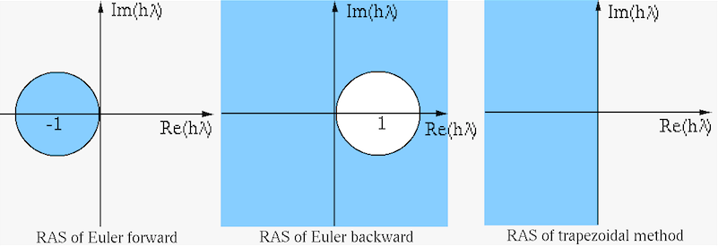
The stability of a specific method can now be measured by applying it to this test equation, in terms of its region of absolute stability (RAS), defined as the region on the complex plane, any value $h\lambda$ in which corresponds to a bounded solution of the differential equation. If, in particular, the entire left-hand plan $Re(h\lambda)<0$ is inside the RAS of a method, then it is absolute stable or A-stable. An A-stable method is always stable, i.e., the numerical solution it generates is bounded, for any step size, so long as $Re(\lambda)<0$, i.e., the true solution of the DE is bounded.

Note that the RAS depends on the product $h\lambda$ (instead of either $h$ or $\lambda$ alone), because a smaller step size $h$ is needed for a larger $\vert Re(\lambda)\vert$ of a more rapidly decaying function $y(t)=y_0e^{\lambda t}$, but a greater step size $h$ can be used for a small $\vert Re(\lambda)\vert$ of a slowly decaying $y(t)$.

The RAS of a general method, such as the multi-step Adams-Moulton method (Eq. (225)), can be obtained by applying it to the test equation $y'=\lambda y$:

$$y_{n+m} = y_{n+m-1}+h\;\sum_{i=n}^{n+m} b_i f_i =y_{n+m-1}+h\;\sum_{i=n}^{n+m} b_i f(t_i,y(t_i))$$

$$= y_{n+m-1}+h\lambda\;\sum_{i=n}^{n+m} b_i y_i$$ (320)

This iteration can be viewed as a homogeneous difference equation:

$$(1-h\lambda b_{n+m})y_{n+m}-(1+h\lambda b_{n+m})y_{n+m-1}+h\lambda\sum_{i=n}^{n+m-2}b_iy_i=0$$ (321)

If we assume $y_n=cz^n$, this equation becomes:

$$(1-h\lambda b_{n+m})cz^{n+m}-(1+h\lambda b_{n+m-1})cz^{n+m-1}+h\lambda\sum_{i=n}^{n+m-2}b_icz^i$$

$$= cz^n [ (1-h\lambda b_{n+m})z^m-(1+h\lambda b_{n+m-1})z^{m-1}+h\lambda\sum_{i=0}^{m-2}b_iz^i ]$$

$$= cz^n\Phi(z,h\lambda)=0$$ (322)

where

$$\Phi(z,h\lambda)=(1-h\lambda b_{n+m})z^m-(1+h\lambda b_{n+m-1})z^{m-1}+h\lambda\sum_{i=0}^{m-2}b_iz^i$$ (323)

is the characteristic polynomial with $m$ roots $z_1,\cdots,z_m$. The solution of the test equation Eq. (320) is the linear combination of $m$ terms of $c_i z_i^n$:

$$y_n=\sum_{i=1}^m c_iz_i^n$$ (324)

where the coefficients $c_0,\cdots,c_{m-1}$ can be determined based on $m$ given initial conditions $y_0,\cdots,y_{m-1}$. For this solution to be bounded we must have $\vert z_i\vert<1$ for all $i=0,\cdots,m-1$.

• Forward Euler's method (Eq. (206), $m=1,\;b_n=1,\;b_{n+1}=0$):
  

  $$y_{n+1} = y_n+h y'_n=y_n+h \lambda y_n=(1+h\lambda) y_n$$

  $$= (1+h\lambda)^2 y_{n-1}=\cdots=(1+h\lambda)^{n+1} y_0$$ (325)

  
  The characteristic equation is

  $$\Phi(z,h\lambda)=z-(1+h\lambda)=0$$ (326)

  We must have $\vert z\vert=\vert 1+h\lambda\vert\le 1$ for the solution to be bounded. Alternatively, we can reach the same result based on the direction observation that the following ratio must be smaller than 1 for the solution to converge:

  $$\bigg\vert\frac{y_{n+1}}{y_n}\bigg\vert=\vert 1+h\lambda\vert \le 1$$ (327)

  This RAS is the unite circle centered at $(-1,\;0)$, the method is not A-stable. On the real axis, we have $\vert 1+h\lambda\vert\le 1$, i.e., $-1<1+h\lambda<1$ or $-2<h\lambda<0$. If $\lambda<0$, i.e., the solution $y(t)=y_0e^{\lambda t}$ exponentially decays to 0, the numerical solution will converge only if $h<-2/\lambda$.

• Backward Euler's method (Eq. (208), $m=1,\;b_n=0,\;b_{n+1}=1$):

  $$y_{n+1}=y_n+h y'_{n+1}=y_n+h \lambda y_{n+1}$$ (328)

  $$\Phi(z,h\lambda)=(1-h\lambda)z-1=0$$ (329)

  For the solution to be bounded, we must have $\vert z\vert=\vert 1/(1-h\lambda)\vert\le 1$, i.e., $1-h\lambda\ge 1$. Alternatively, we can reach the same result based on the direction observation that the following ratio must be smaller than 1 for the solution to converge:

  $$\bigg\vert\frac{y_{n+1}}{y_n}\bigg\vert=\bigg\vert\frac{1}{1-h\lambda}\bigg\vert\le 1, \;\;\;\;\;\; \vert 1-h\lambda\vert \ge 1$$ (330)

  This RAS is the area outside the unite circle centered at $(1,\;0)$. If $\lambda<0$, i.e., the solution $y(t)=y_0e^{\lambda t}$ exponentially decays to 0, the numerical solution will always converge, as no matter how large the step size $h$ may be, $\vert y_{n+1}/y_n\vert$ is always smaller than 1. The method is A-stable.

• The trapezoidal method (Eq. (210)), $m=1,\;b_n=b_{n+1}=1/2$):

  $$y_{n+1}=y_n+h \frac{y'_n+y'_{n+1}}{2}=y_n+\frac{h\lambda(y_n+y_{n+1})}{2}$$ (331)

  $$\Phi(z,h\lambda)=(1-h\lambda/2)z-(1+h\lambda/2)=0$$ (332)

  For the solution to be bounded, we must have $\vert z\vert=\vert(1+h\lambda/2)/(1-h\lambda/2)\vert \le 1$. Alternatively, we can reach the same result based on the direction observation that the following ratio must be smaller than 1 for the solution to converge:

  $$\bigg\vert\frac{y_{n+1}}{y_n}\bigg\vert=\bigg\vert\frac{2+h\lambda}{2-h\lambda}\bigg\vert \le 1$$ (333)

  The inequality holds if $h\lambda < 0$, i.e., the RAS is the entire left-hand plan, the method is A-stable.

  

• Second order Adams-Bashforth method (Eq. (222), $m=2,\;b_{n+1}=0,\;b_{n+1}=3/2,\;b_n=-1/2$):

  $$y_{n+2}=y_{n+1}+h(3f_{n+1}-f_n)/2$$ (334)

  $$\Phi(z,h\lambda)=z^2-(1+3 h\lambda/2)z+h\lambda/2=0$$ (335)

  The two roots are:

  $$z_{1,2}=\frac{1}{2}\left(1+\frac{3}{2}h\lambda\pm\sqrt{1+h\lambda+\frac{9}{4}(h\lambda)^2}\right)$$ (336)

  For the solution to be bounded, we must have $\vert z\vert=1$. In particular, on the real axis, we have

  $$\bigg\vert\frac{1}{2}\left(1+\frac{3}{2}h\lambda\pm\sqrt{1+h\lambda+\frac{9}{4}(h\lambda)^2}\right)\bigg\vert<1$$ (337)

  i.e.,

  $$-2<1+\frac{3}{2}h\lambda\pm\sqrt{1+h\lambda+\frac{9}{4}(h\lambda)^2}<2$$ (338)

  Solving these inequalities, we get $-1<h\lambda<0$.

  Note that for methods of order $m>1$, the condition of stability can no longer be found by solving $y_{n+1}/y_n<1$.

• Runge-Kutta methods:

  As shown in the example in Section , the iterations of RK methods for the test equation $y'=f=\lambda y$ are
  

  $$RK1: y_{n+1}=(1+h\lambda)y_n$$ (339)

  $$RK2: y_{n+1}=[1+h\lambda+(h\lambda)^2/2]y_n$$ (340)

  $$RK3: y_{n+1}=[1+h\lambda+(h\lambda)^2/2+(h\lambda)^3/6]y_n$$ (341)

  $$RK4: y_{n+1}=[1+h\lambda+(h\lambda)^2/2+(h\lambda)^3/6+(h\lambda)^4/24]y_n$$ (342)

  
  For the iteration to converge, we need to have $\vert y_{n+1}\vert/\vert y_n\vert<1$, i.e., the magnitudes of the corresponding polynomial of $h\lambda$ inside the brackets must be smaller than 1. All points of $h\lambda$ that satisfy the inequality above form the RAS on the complex plane, as shown here:

  

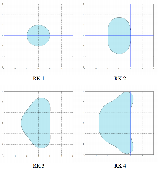
We see that although the RK methods have high order of errors (e.g., RK4 with $O(h^5)$), they are not A-stable, while the implicit backward Euler and trapezoidal methods are both A-stable, even though they have lower order error, as shown in the example of the the previous section.

The discussion above for single-variable linear constant coefficient DEs can be generalized to a multi-variable linear constant coefficient DE systems ${\bf y}'+{\bf Ay}={\bf x}$ with a general solution:

$${\bf y}(t)=\sum_{i=1}^N c_i {\bf v}_ie^{s_it}+{\bf y}_p$$ (343)

which in turn can be further generalized to nonlinear DE systems which can be approximately linearized by dropping all higher order terms in its Taylor expansion except the linear term represented by its Jacobian matrix ${\bf J}$. Then the discussion above in terms of the constant coefficient matrix ${\bf A}$ in a linear system can be generalized to a non-linear system in terms of ${\bf J}$.