Self-Organizing Map (SOM)

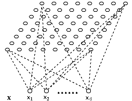
The Self-organizing map (SOM) is a two-layer unsupervised neural network learning algorithm that maps any input pattern presented to its input layer, a vector ${\bf x}=[x_1,\cdots,x_d]^T$ in a d-dimensional feature space, to a set of output nodes that forms a low-dimensional space called feature map, typically a 2-D grid (lattice), although 1-D and 3-D spaces can also be used. A SOM can therefore be considered as a dimensionality reduction method, by which the dataset in the high-dimensional feature space can be visualized and the features and structures of the dataset can be discovered.

The learning rule of the SOM is similar to that of the competitive learning network considered previously in that all output nodes compete based on their activation levels upon the input pattern presented to input nodes of the network. However, different from the competitive learning network where only the winning node gets to modify its weight vector and learn to respond to a cluster of similar patterns individually and independently, here in SOM network all output nodes in the neighborhood of the winning node get to modify their weight vectors and thereby learn to respond collectively to a cluster of similar input patterns. As the result, all output nodes are locked into a continum feature map with smooth and gradual variation in responsive selectivity.

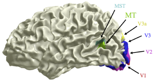
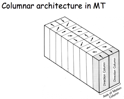
The SOM as a learning algorithm is motivated by the mapping process in the brain, by which signals from various sensory systems (e.g., visual and auditory) are projected (mapped) to different cortical areas and responded to by the neurons wherein in such a way that all neurons in a local cortical area selectively respond to similar stimuli, as shown in the following examples.

Spatially adjacent stimuli are represented and responded to by neurons in adjacent positions in cortex, known as topographic organization.
Sound signals of different frequencies are mapped to the primary auditory cortex where neighboring neurons respond to similar frequencies.
The visual field is topographically projected from the retina to the primary visual cortex V1 where adjacent neurons respond to adjacent areas in the visual field. This projection of the visual field is called retinotopic map.
Visual edges/lines of different orientations are mapped to V1 where neighoring neurons in the columnar architecture respond to similar orientations.
Visual motion of different directions are mapped to the columnar architecture of the middle temporal area (MT or V5) where neighboring neurons respond to similar motion directions.

In a typical SOM network, the output nodes are organized in a 2-D feature map, and the competitive learning algorithm previouisly discussed is modified so that the learning takes place at not only the winning node in the output layer, but also a set of nodes in the neighborhood of the winner. The weight vectors of all such nodes are modified:

$\displaystyle {\bf w}_i^{new}={\bf w}_i^{old}+u_i\eta \,({\bf x}-{\bf w}_i^{old})$

(85)

where

is a weighting function based on the Euclidean distance $d_i$

from the ith node in the neighborhood to the winner in the 2-D feature map, such as a Gaussian function centered at the winner:

$\displaystyle u_i=\exp\left( -\frac{d^2_i}{2\sigma^2} \right) \left\{ \begin{ar... ...for winner with $d_i=0$}\\ <1 & \mbox{for all orther nodes} \end{array}\right.$

(86)

where $\sigma$ is a hyperparameter that controls the width of the Gaussian function. We see that all neurons in the neighborhood of the winner learn from the current input pattern in such a way that their weight vectors are modified to be closer to the input vector in the d-dimensional feature space, but they do so to different extents. Speically, for the winner itself with $d_i=0$

and

, the learning rate for the winner is maximally $\eta$ , while all other nodes with $d_i>0$

also modify their weights but with some lower rates $u_i\eta$ . Those closer to the winner with smaller $d_i$

and thereby greater $u_i$

will learn more than those farther away.

Here are the specific steps of the SOM learning algorithm:

Initialize weights of a set of output nodes arranged in a 2-D map.
Choose randomly an input pattern vector ${\bf x}$ in the high-dimensional feature space and calculate the activation $y_i={\bf w}^T_i{\bf x}$ for each of the output nodes.
Find the winning node with maximum activation and update the weights of all nodes in its neighborhood by Eq. (85).
Go back to step 2 until the feature map is no longer changing or a set maximum number of iterations is reached.

In the training process, both $\sigma$ controlling the size of the neighborhood and $\eta$ for the learning rate will be gradually reduced.

Shown below is the the Matlab code segment for the essential part of the SOM algorithm.

    [d N]=size(X);                         % dataset of N sample vectors
    W=rand(d,M,M);                         % initialization of weights
    for i=1:M
        for j=1:M
            w=reshape(W(:,i,j),[d 1]);
            W(i,j,:)=W(:,i,j)/norm(w);     % normalize all weight vectors
        end
    end
    eta=0.9;                               % initial learning rate
    sgm=M;                                 % width of Gaussian neighborhood
    decay=0.999;                           % rate of decay
    for it=1:nt                            % training iterations
        n=randi([1 N]);                  
        x=X(:,n);                          % pick randomly an input
        amax=-inf;
        for i=1:M                          % find the winner 
            for j=1:M 
                w=reshape(W(:,i,j),[d 1]);
                a=x'*w;                    % activation as inner product
                if a>amax
                    amax=a;  wi=i;  wj=j;  % record winner so far
                end
            end
        end
        for i=1:M
            for j=1:M
                dist=(wi-i)^2+(wj-j)^2;    % distance to winner
                c=exp(-dist/sgm);          % Gaussian weights
                w=reshape(W(:,i,j),[d 1]); % get a weight vector
                w=w+eta*c*(x-w);           % modify weights
                w=w/norm(w);               % normalize weight vectors
                W(:,i,j)=w;                % save modified weight vector
            end
        end
        eta=eta*decay;                     % reduce learning rate
        sgm=sgm*decay;                     % reduce width of Gaussian
    end

Example 1:

This example of “self-organizing map” is how the SOM algorithm got its name. The output nodes are organized into a 2-D map and they learn to respond to the positions of a set of random points ${\bf x}=[x_1,\,x_2]^T$ in a 2-D feature space. The weights of the output nodes are randomly initialized, and then modified during the learning process when the data points are repeatedly presented to the input of the network. When the SOM hase been trained, due to the spatial correlation nature of the algorithm, the output nodes close to each other in the 2-D feature map respond to a set of adjacent data points in the 2-D space, thereby forming a self-organized spatial map, a roughly regular grid.

The 2-D map of the output nodes is visualized as shown in the figure below, where the spatial position of each node is determined by the two components of its weight vector ${\bf w}=[w_1,\,w_2]^T$ treated as its coordinates, and each node is connected to its four neighbors in the 2-D grid to indicate the spatial structure of the feature map.

In this example, the competitive learning is based on the distance between the weight vector ${\bf w}_i$ and the current input ${\bf x}$ , instead of their inner product ${\bf w}^T_i{\bf x}$ . The node with the shortest distance $\vert\vert{\bf w}_i-{\bf x}\vert\vert$ becomes the winner, and its weight vector ${\bf w}$ is pulled even closer to the input, dragging along with it all its neighboring nodes.

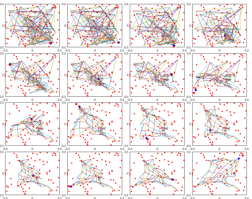
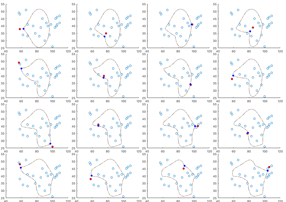
The figure below shows the iterative modification of the weights. In each of the 16 iterations, the output node (blue dot) is closest to the input vector (red dot) and it becomes the winner.

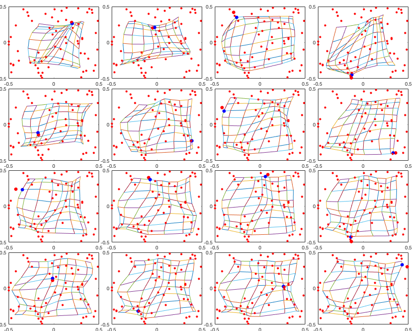
The figure below shows the subsequent iterations in every 50 iterations. The resulting configuration of the output nodes is roughly a regular 2-D grid, a self-organized map in the 2-D feature space.

Example 2:

In this example the output nodes of the SOM are arranged into a 1-D loop and they respond to a set of cities in north America represented by their coordinates (longitudes and latitudes), for the purpose of finding a reasonably short path that goes through all of these cities (the traveling salesman problem). These nodes are visualized in terms of their weight vectors as points in a 2-D map. The weights are initialized to form circle in the map the cities. During the learning iteration when they learn to respond to the 2-D city coordinates as the input, their weights are modified so that they are gradually pulled toward the cities, thereby forming eventually a path through all the cities. In this case, the inner product ${\bf w}_i^T{\bf x}$ is used to determine the winner of each iteration.

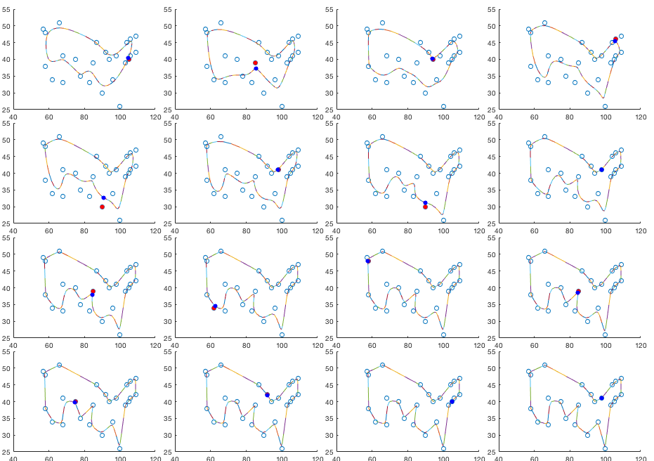
The figure below shows the results of the first 16 iterations:

The figure below shows the subsequent iterations in every 50 iterations. The resulting configuration of the output nodes approaches the desired path that passes through all cities. Although this result does not garantee the path to be the shortest, it is reasonably close to such a solution required by the traveling salesman problem. The final result is unaffected by how the weights are initalized.

Example 3:

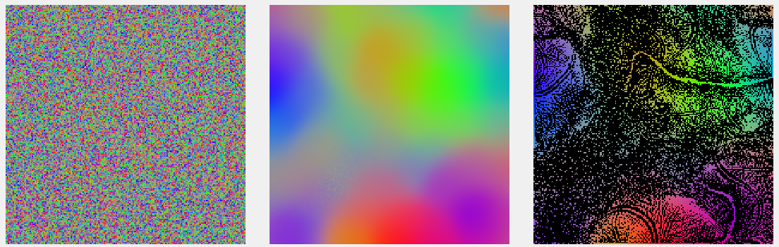
In this example, the output nodes in the 2-D feature map learn to respond to different colors treated as vectors in a 3-D space spanned by the three primary colors red, green and blue (RGB). When the SOM is trained, neighboring output nodes respond to similar colors. Here all input vectors are normalized (the hue of a color is fully determined by the ratios of the three primaries), and so are the weight vectors, which are always renormalized in each iteration.

To visualize the output nodes in the 2-D map, they are color coded based on the three components of their weight vectors treated as the three RGB colors, indicating their favored colors, the color they respond maximally, as shown in the figure below. The left panel is the nodes in the feature map with randomly initialized weights. The middle one shows these nodes after the SOM is fully trained. The right panel shows all the winners during the learning process, all encoded by the input colors they win. The black areas are composed of the output nodes that never win but learn along with their neighboring winners. Interestingly, the winners seem to form some structure in the 2-D space. More detailed discussion can be found here.

More examples of SOM can be found here.