The Fundamental Theorem of Linear Algebra

When solving a linear equation system ${\bf Ax}={\bf b}$ with $M$ equations and $N$ unknowns, the coefficient matrix ${\bf A}$ has $M$ rows and $N$ columns ($M\times N$). We need to answer some questions:

• If the system has fewer equations than unknowns ($M<N$), are there infinite solutions?
• If the system has more equations than unknowns ($M>N$), is there no solution?
• Does the solution exist, i.e., can we find a solution ${\bf x}^*$ so that ${\bf Ax}^*={\bf b}$ holds?
• If a solution exists, is it unique? If it is not unique, how can we find all solutions?
• If no solution exists, can we still find the optimal approximate solution $\hat{\bf x}$ so that the error $\vert\vert{\bf e}\vert\vert=\vert\vert{\bf A}\hat{\bf x}-{\bf b}\vert\vert$ is minimized?

The fundamental theorem of linear algebra can reveal the structure of the solutions of any given linear system ${\bf Ax}={\bf b}$, and thereby answer all questions above.

The $M\times N$ coefficient matrix ${\bf A}\in\mathbb{R}^{M\times N}$ can be expressed in terms of either its $N$ M-D column vectors ${\bf c}_j$ or its $M$ N-D row vectors ${\bf r}_i^T$:

$${\bf A}=\left[\begin{array}{ccc}a_{11}&\cdots&a_{1N}\\ \vdots&\d... ...N] =\left[\begin{array}{c}{\bf r}^T_1\\ \vdots\\ {\bf r}^T_M\end{array}\right],$$ (134)

$${\bf A}^T=\left[\begin{array}{ccc}a_{11}&\cdots&a_{M1}\\ \vdots&... ..._M] =\left[\begin{array}{c}{\bf c}^T_1\\ \vdots\\ {\bf c}^T_N\end{array}\right]$$ (135)

where ${\bf r}_i,\;(i=1,\cdots,M)$ and ${\bf c}_j,\;(j=1,\cdots,N)$ are respectively the ith row vector and jth column vector (all vectors are assumed to be vertical):

$${\bf c}_j=\left[\begin{array}{c}a_{1j}\\ \vdots\\ a_{Mj}\end{arra... ...}_i=\left[\begin{array}{c}a_{i1}\\ \vdots\\ a_{iN}\end{array}\right] \;\;\;\;\; \;\;\; {\bf r}_i^T=[a_{i1},\cdots,a_{iN}]$$ (136)

In general a function $y=f(x)$ can be represented by $f:\;X\rightarrow Y$, where

• $X$ is the domain of the function, the set of all input or argument values;
• $Y$ the codomain of the function, the set into which all outputs of the function are constrained to fall;
• the set of $f(x)$ for all $x\in X$ is the image of the function, a subset of the codomain.

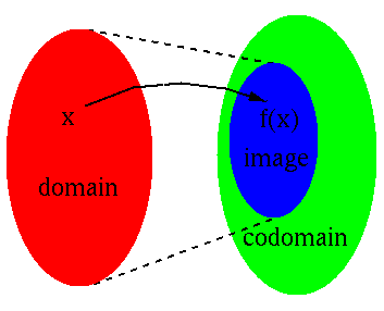
The matrix ${\bf A}$ can be considered as a function, a linear transformation ${\bf f}({\bf x})={\bf Ax}$, which maps an N-D vector ${\bf x}\in \mathbb{R}^N$ in the domain of the function into an M-D vector ${\bf Ax}\in R^M$ in the codomain of the function. The fundamental theorem of linear algebra concerns the following four subspaces associated with any $M\times N$ matrix ${\bf A}$ with rank $R=rank({\bf A})\le \min(M,\,N)$ (i.e., ${\bf A}$ has $R$ independent columns and rows).

• The column space (image) of ${\bf A}$ is a space spanned by its $N$ M-D column vectors (of which $R\le N$ are independent):

  $$C({\bf A})=span({\bf c}_1,\cdots,{\bf c}_N) \subseteq \mathbb{R}^M$$ (137)

  which is an R-D subspace of $\mathbb{R}^M$ composed of all possible linear combinations of its $N$ column vectors:

  $$x_1{\bf c}_1+\cdots+x_N{\bf c}_N=[{\bf c_1},\cdots,{\bf c}_N] \le... ...begin{array}{c}x_1\\ \vdots\\ x_N\end{array}\right] ={\bf A}{\bf x}\;\;\;\;\;\; \mbox{(for any ${\bf x}\in\mathbb{R}^N$)}$$ (138)

  The column space $C({\bf A})$ is the image of the linear transformation ${\bf f}({\bf x})={\bf Ax}$, and the equation ${\bf Ax}={\bf b}$ is solvable if and only if ${\bf b}\in C({\bf A})$. The dimension of the column space is the rank of ${\bf A}$, $dim\,C({\bf A})=rank({\bf A})=R$.

• The row space of ${\bf A}$ (the column space of ${\bf A}^T$) is a space spanned by its $M$ N-D row vectors (of which $R\le M$ are independent):

  $$R({\bf A})=span({\bf r}_1,\cdots,{\bf r}_M) \subseteq \mathbb{R}^N$$ (139)

  which is an R-D subspace of $\mathbb{R}^N$ composed of all possible linear combinations of its $M$ row vectors:

  $$y_1{\bf r}_1+\cdots+y_M{\bf r}_N=[{\bf r_1},\cdots,{\bf r}_M] \le... ...gin{array}{c}y_1\\ \vdots\\ y_M\end{array}\right] ={\bf A}^T{\bf y}\;\;\;\;\;\; \mbox{(for any ${\bf y}\in \mathbb{R}^M$)}$$ (140)

  The row space $R({\bf A})$ is the image of the linear transformation ${\bf f}({\bf y})={\bf A}^T{\bf y}$, and the equation ${\bf A}^T{\bf y}={\bf c}$ is solvable if and only if ${\bf c}\in R({\bf A})$. As the rows and columns in ${\bf A}$ are respectively the columns and rows in ${\bf A}^T$, the row space of ${\bf A}$ is the column space of ${\bf A}^T$, and the column space of ${\bf A}$ is the row space of ${\bf A}^T$:

  $$R({\bf A})=C({\bf A}^T),\;\;\;\;\;\;\;\;\;\;C({\bf A})=R({\bf A}^T)$$ (141)

  The rank $R=rank({\bf A})$ is the number of linearly independent rows and columns of ${\bf A}$, i.e., the row space and the column space have the same dimension, both equal to the rank of ${\bf A}$:

  $$dim\,C({\bf A})=dim\,R({\bf A})=rank({\bf A})=R$$ (142)

• The null space (kernel) of ${\bf A}$, denoted by $N({\bf A})$, is the set of all N-D vectors ${\bf x}$ that satisfy the homogeneous equation

  $${\bf A}{\bf x}=\left[\begin{array}{c}{\bf r}^T_1\\ \vdots\\ {\bf r}^T_M\end{array}\right] {\bf x}={\bf0},\;\;\;\;\;\; \;\;\;\;\;\; {\bf r}^T_i{\bf x}=0\;\;\;(i=1,\cdots,M)$$ (143)

  i.e.,

  $$N({\bf A})=\{ {\bf x}\in\mathbb{R}^N \vert {\bf A}{\bf x} ={\bf0} \}\subseteq \mathbb{R}^N$$ (144)

  In particular, when ${\bf x}={\bf0}$, we get ${\bf A}{\bf x}={\bf0}$, i.e., the origin ${\bf0}\in N({\bf A})$ is in the null space.

  As ${\bf r}^T_i{\bf x}=0$ for any ${\bf x}\in N({\bf A})$ and ${\bf r}_i\in R({\bf A})$, we see that the null space $N({\bf A})$ and the row space $R({\bf A})=C({\bf A}^T)$ are orthogonal to each other, $N({\bf A}) \perp R({\bf A})$.

  The dimension of the null space is called the nullity of ${\bf A}$: $dim\;N({\bf A})=nullity({\bf A})$. The rank-nullity theorem states the sum of the rank and the nullity of an $M\times N$ matrix ${\bf A}$ is equal to $N$:

  $$({\bf A})+nullity({\bf A})=dim\;R({\bf A})+dim\;N({\bf A})=N$$ (145)

  We therefore see that $R({\bf A})$ and $N({\bf A})$ are two mutually exclusive and complementary subspaces of $\mathbb{R}^N$:

  $$R({\bf A}) \perp N({\bf A}),\;\;\;\; R({\bf A}) \cap N({\bf A})=\emptyset,\;\;\;\;\; R({\bf A}) \oplus N({\bf A})=\mathbb{R}^N$$ (146)

  i.e., they are orthogonal complement of each other, denoted by

  $$N({\bf A})=R({\bf A})^\perp,\;\;\;\;R({\bf A})=N({\bf A})^\perp$$ (147)

  Any N-D vector ${\bf x}\in \mathbb{R}^N$ is in either of the two subspaces $R({\bf A})$ and $N({\bf A})$.

• The null space of ${\bf A}^T$ (left null space of ${\bf A})$, denoted by $N({\bf A}^T)$, is the set of all M-D vectors ${\bf y}$ that satisfy the homogeneous equation

  $${\bf A}^T{\bf y}=[{\bf c}_1,\cdots,{\bf c}_N]^T{\bf y} =\left[\be... ...\bf c}^T_1\\ \vdots\\ {\bf c}^T_N\end{array}\right] {\bf y}={\bf0},\;\;\;\;\;\; \;\;\;\;\;\; {\bf c}^T_j{\bf y}=0,\;\;\;(j=1,\cdots,N)$$ (148)

  i.e.,

  $$N({\bf A}^T)=\{ {\bf y}\in\mathbb{R}^M \vert {\bf A}^T{\bf y} ={\bf0} \}\subseteq \mathbb{R}^M$$ (149)

  As all ${\bf y}\in N({\bf A}^T)$ are orthogonal to ${\bf c}_i\in C({\bf A})$, $N({\bf A}^T)$ is orthogonal to the column space $C({\bf A})=R({\bf A}^T)$:

  $$N({\bf A}^T) \perp C({\bf A}),\;\;\;\;\;\;\;N({\bf A}^T) \perp R({\bf A}^T)$$ (150)

  We see that $C({\bf A})$ and $N({\bf A}^T)$ are two mutually exclusive and complementary subspaces of $\mathbb{R}^M$:
  

  $$C({\bf A}) \perp N({\bf A}^T),\;\;\;\;\; C({\bf A}) \cap N({\bf A}^T)=\emptyset,\;\;\;\;\; C({\bf A}) \oplus N({\bf A}^T)=R^M,$$

  $$N({\bf A}^T)=C({\bf A})^\perp,\;\;\;\;C({\bf A})=N({\bf A}^T)^\perp$$ i.e. (151)

  
  Any M-D vector ${\bf y}\in \mathbb{R}^M$ is in either of the two subspaces $C({\bf A})$ and $N({\bf A}^T)$.

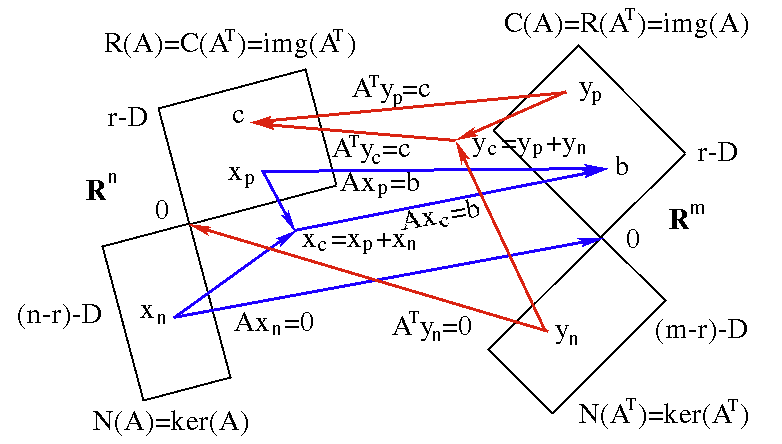
The four subspaces are summarized in the figure below, showing the domain $\mathbb{R}^N=R({\bf A})\oplus N({\bf A})$ (left) and the codomain $\mathbb{R}^M=C({\bf A})\oplus N({\bf A}^T)$ (right) of the linear mapping ${\bf Ax}={\bf b}$, where

• ${\bf x}_p\in R({\bf A})$ is the particular solution that is mapped to ${\bf Ax}_p={\bf b}\in C({\bf A})$, the image of $f({\bf x})={\bf Ax}$;
• ${\bf x}_h\in N({\bf A})$ is a homogeneous solution that is mapped to ${\bf Ax}_h={\bf0}\in \mathbb{R}^M$;
• ${\bf x}_c={\bf x}_p+{\bf x}_h$ is the complete solution that is mapped to ${\bf Ax}_c={\bf b}\in C({\bf A})$.

On the other hand, ${\bf y}_p\in C({\bf A})=R({\bf A}^T)$, ${\bf y}_h\in N({\bf A}^T)$, and ${\bf y}_c={\bf y}_p+{\bf y}_h$ are respectively the particular, homogeneous and complete solutions of ${\bf A}^T{\bf y}={\bf c}$. Here we have assumed ${\bf b}\in C({\bf A})$ and ${\bf c}\in R({\bf A})$, i.e., both ${\bf Ax}={\bf b}$ and ${\bf A}^T{\bf y}={\bf c}$ are solvable. We will also consider the case where ${\bf b}\notin C({\bf A})$ later.

Based on the rank $R=rank({\bf A}$ of any $M\times N$ matrix ${\bf A}$, we can determine the dimensionalities of the four associated spaces and the existence and uniqueness of solution of the system ${\bf Ax}={\bf b}$:

• If $R=M=N$, $N({\bf A})=N({\bf A}^T)=\emptyset$, then ${\bf b}\in C({\bf A})=\mathbb{R}^M$, unique solution exists;
• If $R=M<N$, $N({\bf A})\ne \emptyset$, $N({\bf A}^T)=\emptyset$, then ${\bf b}\in C({\bf A})=\mathbb{R}^M$, infinite solutions exist;
• If $R=N<M$, $N({\bf A})=\emptyset$, $N({\bf A}^T)\ne \emptyset$, then unique solution exists if ${\bf b}\in C({\bf A})\subset\mathbb{R}^M$, but no solution otherwise;
• If $R<\min(M,N)$, $N({\bf A})\ne \emptyset$, $N({\bf A}^T)\ne \emptyset$, then infinite solutions exist if ${\bf b}\in C({\bf A})\subset\mathbb{R}^M$, but no solution otherwise.

We now consider specifically how to find the solutions of the system ${\bf Ax}={\bf b}$ in light of the four subspaces of ${\bf A}$ defined above, through the examples below.

Example 1:

Solve the homogeneous equation system:

$${\bf A}{\bf x}=\left[\begin{array}{ccc}1&2&5\\ 2&3&8\\ 3&1&5\end{... ..._3\end{array}\right] =\left[\begin{array}{c}0\\ 0\\ 0\end{array}\right] ={\bf0}$$ (152)

We first convert ${\bf A}$ into the rref:

$$\left[\begin{array}{ccc}1&2&5\\ 2&3&8\\ 3&1&5\end{array}\right] \... ... x_2\\ x_3\end{array}\right] =\left[\begin{array}{c}0\\ 0\\ 0\end{array}\right]$$

The $R=rank({\bf A})=2$ columns in the rref containing a single 1, called a pivot, are called the pivot columns, and the rows containing a pivot are called the pivot rows. Here, $R=2<M=N=3$, i.e., ${\bf A}$ is a singular matrix. The two pivot rows ${\bf r}_1^T=[1,\;0,\;1]$ and ${\bf r}_2^T=[0,\;1,\;2]$ can be used as the basis vectors that span the row space $R({\bf A})$:

$$R({\bf A})=c_1{\bf r}_1+c_2{\bf r}_2 =c_1\left[\begin{array}{r}1\\ 0\\ 1\end{array}\right] +c_2\left[\begin{array}{r}0\\ 1\\ 2\end{array}\right]$$

Note that the pivot columns of the rref do not span the column space $C({\bf A})$, as the row reduction operations do not preserve the columns of ${\bf A}$. But they indicate the corresponding columns ${\bf c}_1=[1\;2\;3]^T$ and ${\bf c}_2=[2\;3\;1]^T$ in the original matrix ${\bf A}$ can be used as the basis that spans $C({\bf A})$. In general the bases of the row and column spaces so obtained are not orthogonal.

The $R$ pivot rows are the independent equations in the system of $M$ equations, and the variables corresponding to the pivot columns (here $x_1$ and $x_2$) are the pivot variables. The remaining $M-R$ non-pivot rows containing all zeros are not independent, and the variables corresponding to the non-pivot rows are free variables (here $x_3$), which can take any values.

From the rref form of the equation, we get

$$x_1+x_3=0,\;\;\;x_2+2x_3=0$$

If we let the free variable $x_3=1$, then we can get the two pivot variables $x_1=-1$ and $x_2=-2$, and a special homogeneous solution ${\bf x}_h=[-1\;-2\;1]^T$ as a basis vector that spans the 1-D null space $N({\bf A})$. However, as the free variable $x_3$ can take any value $c$, the complete solution is the entire 1-D null space:

$$N({\bf A})=c {\bf x}_h=c\left[\begin{array}{r}-1\\ -2\\ 1\end{array}\right]$$

Example 2:

Solve the non-homogeneous equation with the same coefficient matrix ${\bf A}$ used in the previous example:

$${\bf A}{\bf x}= \left[\begin{array}{ccc}1&2&5\\ 2&3&8\\ 3&1&5\end... ...end{array}\right] =\left[\begin{array}{c}19\\ 31\\ 22\end{array}\right]={\bf b}$$

We use Gauss-Jordan elimination to solve this system:

$$[\begin{array}{cc}{\bf A}&{\bf b}\end{array}] =\left[\begin{array... ...ow \left[\begin{array}{rrr\vert r}1&0&1&5\\ 0&1&2&7\\ 0&0&0&0\end{array}\right]$$

The $R=2$ pivot rows correspond to the independent equations in the system, i.e., $rank({\bf A})=2$, while the remaining $M-R=1$ non-pivot row does not play any role as they map any ${\bf x}$ to ${\bf0}$. As ${\bf A}$ is singular, ${\bf A}^{-1}$ does not exist. However, we can find the solution based on the rref of the system, which can also be expressed in block matrix form:

$$\left[\begin{array}{rrr}1&0&1\\ 0&1&2\\ 0&0&0\end{array}\right] \... ...ray}\right]= \left[\begin{array}{c}5\\ 7\\ 0\end{array}\right] \;\;\;\;\;\;\;\; \;\;\;\;\;\;\;\; \left[\begin{array}{rr}{\bf I}&{\bf F}\\ {\bf0}&... ...}\end{array}\right] =\left[\begin{array}{c}{\bf b}_1\\ {\bf0}\end{array}\right]$$

where

$${\bf I}=\left[\begin{array}{cc}1&0\\ 0&1\end{array}\right],\;\;\;... ...{free}=x_3,\;\;\;\;\;\; {\bf b}_1=\left[\begin{array}{c}5\\ 7\end{array}\right]$$

Solving the matrix equation above for ${\bf x}_{pivot}$, we get

$${\bf I}{\bf x}_{pivot}+{\bf F}{\bf x}_{free}={\bf b}_1,\;\;\;\;\;... ...{c}5\\ 7\end{array}\right] +\left[\begin{array}{c}-1\\ -2\end{array}\right] x_3$$

If we let ${\bf x}_{free}=x_3=0$, we get a particular solution ${\bf x}_p=[5\;7\;0]^T$, which can be expressed as a linear combination of ${\bf r}_1$ and ${\bf r}_2$ that span $R({\bf A})$, and ${\bf x}_h$ that span $N({\bf A})$:

$${\bf x}_p=\left[\begin{array}{c}5\\ 7\\ 0\end{array}\right] =\fra... ...{array}\right] -\frac{19}{6}\left[\begin{array}{r}-1\\ -2\\ 1\end{array}\right]$$

We see that this solution is not entirely in the row space $R({\bf A})$. In general, this is the case for all particular solutions so obtained.

Having found both the particular solution ${\bf x}_p$ and the homogeneous solution ${\bf x}_h$, we can further find the complete solution ${\bf x}_c$ as the sum of ${\bf x}_p$ and the entire null space spanned by ${\bf x}_h$:

$${\bf x}_c=\left[\begin{array}{c}5\\ 7\\ 0\end{array}\right] +c \l... ...ay}{r}-1\\ -2\\ 1\end{array}\right] ={\bf x}_p+c {\bf x}_h={\bf x}_p+N({\bf A})$$

Based on different constant $c$, we get a set of equally valid solutions. For example, if $c=0,1,2$, then we get

$${\bf x}_0=\left[\begin{array}{c}5\\ 7\\ 0\end{array}\right],\;\;\... ...ay}\right],\;\;\;\; {\bf x}_2=\left[\begin{array}{c}3\\ 3\\ 2\end{array}\right]$$

These solutions have the same projection onto the row space $R({\bf A})$, i.e., they have the same projections onto the two basis vectors ${\bf r}_1$ and ${\bf r}_2$ that span $R({\bf A})$:

$${\bf x}_0^T{\bf r}_1={\bf x}_1^T{\bf r}_1={\bf x}_2^T{\bf r}_1=5, \;\;\;\;\;\;\;\; {\bf x}_0^T{\bf r}_2={\bf x}_1^T{\bf r}_2={\bf x}_2^T{\bf r}_2=7$$

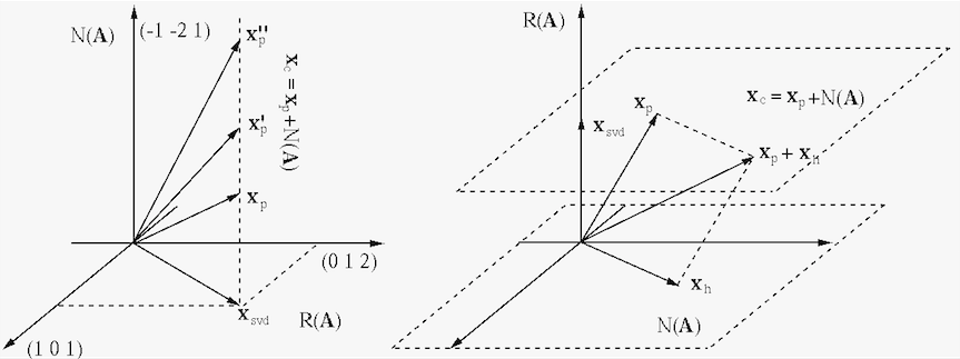
The figure below shows how the complete solution ${\bf x}_c$ can be obtained as the sum of a particular solution ${\bf x}_p$ in $R({\bf A})$ and the entire null space $N({\bf A})$. Here $N=3$ and space $\mathbb{R}^3$ is composed of $R({\bf A})$ and $N({\bf A})$, respectively 2-D and 1-D on the left, but 1-D and 2-D on the right. In either case, the complete solution is any particular solution plus the entire null space, the vertical dashed line on the left, the top dashed plane on the right. All points on the vertical line or top satisfy the equation system, as they are have the same projection onto the row space $R({\bf A})$.

If the right hand side is ${\bf b}'=[19,\,31,\,20]^T$, then the rref of the equation becomes:

$$\left[\begin{array}{rrr}1&0&1\\ 0&1&2\\ 0&0&0\end{array}\right] \... ... x_2\\ x_3\end{array}\right]= \left[\begin{array}{c}5\\ 7\\ 2\end{array}\right]$$

The non-pivot row is an impossible equation $0=2$, indicating that no solution exists, as ${\bf b}'\notin C({\bf A})$ is not in the column space spanned by ${\bf r}_1=[1\;0\;1]^T$ and ${\bf r}_2=[0\;1\;2]^T$.

Example 3: Find the complete solution of the following linear equation system:

$${\bf A}{\bf x}=\left[\begin{array}{rccc}1&2&3&4\\ 4&3&2&1\\ -2&1&... ...4\end{array}\right] =\left[\begin{array}{r}3\\ 2\\ 4\end{array}\right] ={\bf b}$$

This equation can be solved in the following steps:

• Construct the augmented matrix and then convert it to the rref form:
  

  $$\left[\begin{array}{rrrr\vert r}1&2&3&4&3\\ 4&3&2&1&2\\ -2&1&4&7&4\end{array}\right] \rightarrow \left[\begin{array}{rrrr\vert r}1&2&3&4&3\\ 0&-5&-10&-15&-10\\ 0&... ...t[\begin{array}{rrrr\vert r}1&2&3&4&3\\ 0&1&2&3&2\\ 0&0&0&0&0\end{array}\right]$$

  $$\rightarrow \left[\begin{array}{rrrr\vert r}1&0&-1&-2&-1\\ 0&1&2&3&2\\ 0&0&0&... ...y}{rr\vert r}{\bf I}&{\bf F}&{\bf b_1}\\ {\bf0}&{\bf0}&{\bf0}\end{array}\right]$$

  
  The two pivot rows ${\bf r}_1^T=[1\;0\;-1\;-2]$ and ${\bf r}_2^T=[0\;1\;2\;3]$ in the rref span $R({\bf A})$, and the two columns in the original matrix ${\bf A}$ corresponding to the pivot columns in the rref, $[1\;4\;-2]^T$ and $[2\;3\;1]^T$ could be used as the basis vectors that span $C({\bf A})$.

  The equation system can be represented in block matrix form:

  $$\left[\begin{array}{rr}{\bf I}&{\bf F}\\ {\bf0}&{\bf0}\end{array}... ...f\end{array}\right]= \left[\begin{array}{c}{\bf b_1}\\ {\bf0}\end{array}\right]$$

  where

  $${\bf I}=\left[\begin{array}{cc}1&0\\ 0&1\end{array}\right],\;\;\;... ...ray}\right],\;\;\;\;\; {\bf b}_1=\left[\begin{array}{r}-1\\ 2\end{array}\right]$$

  Multiplying out we get

  $${\bf x}_p+{\bf F}{\bf x}_f={\bf b}_1$$

• Find the homogeneous solution for equation ${\bf A}{\bf x}={\bf0}$ by setting ${\bf b}_1={\bf0}$:

  $${\bf I}{\bf x}_p+{\bf F}{\bf x}_f={\bf0}, \;\;\;\; \;\;\;\;\; {\bf x}_p=\left[\begin{array}{c}x_1\\ x_2\end{array}\r... ...1&2\\ -2&-3\end{array}\right] \left[\begin{array}{r}x_3\\ x_4\end{array}\right]$$

  We let ${\bf x}_f$ be either of the two standard basis vectors ${\bf x}_f=[x_3,\;x_4]^T=[1\;0]^T$ and ${\bf x}_f=[x_3,\;x_4]^T=[0\;1]^T$ of the null space $N({\bf A})$, and get

  $${\bf x}_p=\left[\begin{array}{c}x_1\\ x_2\end{array}\right] =\left[\begin{array}{r}1\\ -2\end{array}\right] \;\;\;\;\; \;\;\;\;\; \left[\begin{array}{r}2\\ -3\end{array}\right]$$

  and the two corresponding homogeneous solutions:

  $${\bf x}_{h1}=\left[\begin{array}{c}x_1\\ x_2\\ x_3\\ x_4\end{arra... ...\ x_4\end{array}\right] =\left[\begin{array}{r}2\\ -3\\ 0\\ 1\end{array}\right]$$

• Find the particular solution of the non-homogeneous equation ${\bf A}{\bf x}={\bf b}$ by setting ${\bf x}_f={\bf0}$

  $${\bf I}{\bf x}_p+{\bf F}{\bf x}_f={\bf x}_p={\bf b}_1, \;\;\;\; \;\;\;\;\; \left[\begin{array}{c}x_1\\ x_2\end{array}\right] =\left[\begin{array}{r}-1\\ 2\end{array}\right] \;\;\;\;\; \;\;\;\;\;\;\; {\bf x}_p=\left[\begin{array}{r}-1\\ 2\\ 0\\ 0\end{array}\right]$$

• Find the complete solution:

  $${\bf x}_c={\bf x}_p+N({\bf A}) ={\bf x}_p+c_1{\bf x}_{h1}+c_2{\bf... ... 0\end{array}\right] +c_2\left[\begin{array}{r}2\\ -3\\ 0\\ 1\end{array}\right]$$

If the right-hand side is ${\bf b}'=[1,\;3,\;5]^T$, then the row reduction of the augmented matrix yields:

$$\left[\begin{array}{rrrr\vert r}1&2&3&4&1\\ 4&3&2&1&3\\ -2&1&4&7&... ...egin{array}{rrrr\vert r}1&2&3&4&1\\ 0&1&2&3&0.2\\ 0&0&0&0&1.2\end{array}\right]$$

The equation corresponding to the last non-pivot row is $0=1.2$, indicating the system is not solvable (even though the coefficient matrix does not have full rank), because ${\bf b}'\notin C({\bf A})$ is not in the column space.

Example 4: Consider the linear equation system with a coefficient matrix ${\bf A}^T$, the transpose of ${\bf A}$ used in the previous example:

$${\bf A}^T{\bf y}=\left[\begin{array}{rrr}1&4&-2\\ 2&3&1\\ 3&2&4\\... ...array}\right] =\left[\begin{array}{c}3\\ 11\\ 19\\ 27\end{array}\right]={\bf c}$$

• Convert the augmented matrix into the rref form:

  $$\left[\begin{array}{rrr\vert r}1&4&-2&3\\ 2&3&1&11\\ 3&2&4&19\\ 4... ...gin{array}{rrr\vert r}1&0&2&7\\ 0&1&-1&-1\\ 0&0&0&0\\ 0&0&0&0\end{array}\right]$$

  The two pivot rows ${\bf r}^T_1=[1\;0\;2]$ and ${\bf r}^T_2=[0\;1\;-1]$ are the basis vectors that span $R({\bf A}^T)=C({\bf A})$. The two vectors that span $C({\bf A})$ found in Example 3 can be expressed as linear combinations of ${\bf r}_1$ and ${\bf r}_2$, $[1\;4\;-2]^T={\bf r}_1+4{\bf r}_2$ and $[2\;3\;1]^T=2{\bf r}_1+3{\bf r}_2$, i.e., either of the two pairs can be used as the basis that span $C({\bf A})$.

  Based on the rref above, the equation system can now be written as

  $$\left[\begin{array}{cc}{\bf I}&{\bf F}\\ {\bf0}&{\bf0}\end{array}... ...f\end{array}\right]= \left[\begin{array}{r}{\bf c}_1\\ {\bf0}\end{array}\right]$$

  where

  $${\bf I}=\left[\begin{array}{cc}1&0\\ 0&1\end{array}\right],\;\;\;... ...bf y}_f=y_3,\;\;\;\;\; {\bf c}_1=\left[\begin{array}{r}7\\ -1\end{array}\right]$$

  Multiplying out we get

  $${\bf I}{\bf y}_p+{\bf F}{\bf y}_f={\bf c}_1$$ (153)

• Find the homogeneous solution for ${\bf A}^T{\bf y}={\bf c}={\bf0}$ by setting ${\bf c}={\bf0}$ and thereby ${\bf c}_1={\bf0}$. We let the free variable ${\bf y}_f=y_3=1$ and get

  $${\bf I}{\bf y}_p+{\bf F}{\bf y}_f={\bf0}, \;\;\;\;\; \;\;\;\;\; {\bf y}_p=-{\bf F}{\bf y}_f =\left[\begin{array}{c}y_1... ...nd{array}\right]y_3 =\left[\begin{array}{r}-2\\ 1\end{array}\right], \;\;\;\;\; \;\;\;\;\; {\bf y}_h=\left[\begin{array}{r}-2\\ 1\\ 1\end{array}\right]$$

• Find the particular solution of the non-homogeneous equation ${\bf A}^T{\bf y}={\bf c}\ne {\bf0}$ by setting ${\bf y}_f=y_3=0$:

  $${\bf I}{\bf y}_p+{\bf F}{\bf y}_f={\bf y}_p ={\bf c}_1=\left[\begin{array}{r}7\\ -1\end{array}\right], \;\;\;\;\; \;\;\;\;\; {\bf y}_p=\left[\begin{array}{r}7\\ -1\\ 0\end{array}\right]$$ (154)

• Find the complete solution:

  $${\bf y}_c={\bf y}_p+N({\bf A}^T)={\bf y}_p+c y_3 =\left[\begin{ar... ...\ -1\\ 0\end{array}\right]+c \left[\begin{array}{r}-2\\ 1\\ 1\end{array}\right]$$

If the right-hand side is ${\bf c}'=[1,\;1,\;2,\;3]^T$,

$$\left[\begin{array}{rrr\vert r}1&4&-2&1\\ 2&3&1&1\\ 3&2&4&2\\ 4&1... ...n{array}{rrr\vert r}1&4&-2&1\\ 0&1&-1&1/5\\ 0&0&0&1\\ 0&0&0&2\end{array}\right]$$

indicating the system is not solvable, as this ${\bf c}'\notin C({\bf A}^T)=R({\bf A})$, i.e., it is not in the column space of ${\bf A}^T$ or row space of ${\bf A}$.

In the two examples above, we have obtained all four subspaces associated with this matrix ${\bf A}$ with $M=3$, $N=4$, and $R=2$, in terms of the bases that span the subspaces:

1. The row space $R({\bf A})=C({\bf A}^T)$ is an R-D subspace of $\mathbb{R}^4$, spanned by the $R=2$ pivot rows of the rref of ${\bf A}$:

   $$R({\bf A})=C({\bf A}^T)= span\left(\left[\begin{array}{r}1\\ 0\\ ... ...end{array}\right], \left[\begin{array}{c}0\\ 1\\ 2\\ 3\end{array}\right]\right)$$

2. The null space $N({\bf A})$ is an (N-R)-D subspace of $\mathbb{R}^4$ spanned by the $N-R$ independent homogeneous solutions:

   $$N({\bf A})=span\left(\left[\begin{array}{r}1\\ -2\\ 1\\ 0\end{array}\right], \left[\begin{array}{r}2\\ -3\\ 0\\ 1\end{array}\right] \right)$$

   Note that the basis vectors of $N({\bf A})$ are indeed orthogonal to those of $R({\bf A})$.
3. The column space of ${\bf A}$ is the same as the row space of ${\bf A}^T$, which is the R-D subspace of $R^3$ spanned by the two pivot rows of the rref of ${\bf A}^T$.

   $$C({\bf A})=R({\bf A}^T)=span\left(\left[\begin{array}{c}1\\ 0\\ 2\end{array}\right], \left[\begin{array}{r}0\\ 1\\ -1\end{array}\right]\right)$$

4. The left null space $N({\bf A}^T)$ is a (M-R)-D subspace of $\mathbb{R}^3$ spanned by the homogeneous solutions (here one $3-2=1$ solution):

   $$N({\bf A}^T)=span\left(\left[\begin{array}{r}-2\\ 1\\ 1\end{array}\right] \right) =c\;\left[\begin{array}{r}-2\\ 1\\ 1\end{array}\right]$$

   Again note that the basis vectors of $N({\bf A}^T)$ are orthogonal to those of $C({\bf A})$.

In general, here are the ways to find the bases of the four subspaces:

• The basis vectors of $R({\bf A})$ are the pivot rows of the rref of ${\bf A}$.
• The basis vectors of $C({\bf A})$ are the pivot rows of the rref of ${\bf A}^T$.
• The basis vectors of $N({\bf A})$ are the independent homogeneous solutions of ${\bf Ax}={\bf0}$. To find them, reduce ${\bf A}$ to the rref, identify all free variables ${\bf x}_f$ corresponding to non-pivot columns, set one of them to 1 and the rest to 0, solve homogeneous system ${\bf A}{\bf x}={\bf0}$ to find the pivot variables ${\bf x}_p$ to get one basis vector. Repeat the process for each of the free variables to get all basis vectors.
• The basis vectors of $R({\bf A}^T)$ can be obtained by doing the same as above for ${\bf A}^T$.

Note that while the basis of $R({\bf A})$ are the pivot rows of the rref of ${\bf A}$, as its rows are equivalent to those of ${\bf A}$, the pivot columns of the rref basis of $C({\bf A})$ are not the basis of $C({\bf A})$, as the columns of ${\bf A}$ have been changed by the row deduction operations and are therefore not equivalent to the columns of the resulting rref. The columns in ${\bf A}$ corresponding to the pivot columns in the rref could be used as the basis of $C({\bf A})$. Alternatively, the basis of $C({\bf A})$ can be obtained from the rref of ${\bf A}^T$, as its rows are equivalent to those of ${\bf A}^T$, which are the columns of ${\bf A}$.

We further make the following observations:

• The basis vectors of each of the four subspaces are independent, the basis vectors of $R({\bf A})$ and $N({\bf A})$ are orthogonal, and $dim\;R({\bf A})+dim\;N({\bf A})=M$. Similarly, the basis vectors of $C({\bf A})$ and $N({\bf A}^T)$ are orthogonal, and $dim\;C({\bf A})+dim\;N({\bf A}^T)=N$. In other words, the four subspaces indeed satisfy the following orthogonal and complementary properties:

  $$C({\bf A})\perp N({\bf A}^T),\;\;\;\;R({\bf A})\perp N({\bf A}), ... ...\;\;\;C({\bf A})\oplus N({\bf A}^T)=R^3,\;\;\;\;R({\bf A})\oplus N({\bf A})=R^4$$ (155)

  i.e., they are orthogonal complements: $C({\bf A})=N({\bf A})^\perp,\;\;\;\;R({\bf A})=N({\bf A})^\perp$.

• For ${\bf Ax}={\bf b}$ to be solvable, the constant vector ${\bf b}$ on the right-hand side must be in the column space, ${\bf b}\in C({\bf A})$. Otherwise the equation is not solvable, even if $R<M<N$. Similarly, for ${\bf A}^T{\bf x}={\bf c}$ to be solvable, ${\bf c}$ must be in the row space ${\bf c}\in R({\bf A})$. In the examples above, both ${\bf b}$ and ${\bf c}$ are indeed in their corresponding column spaces:

  $${\bf b}=\left[\begin{array}{r}3\\ 2\\ 4\end{array}\right] =3\left... ...}\right] +11\left[\begin{array}{r}0\\ 1\\ 2\\ 3\end{array}\right]\in R({\bf A})$$ (156)

  But as ${\bf b}=[1,\;3,\;5]^T\notin C({\bf A})$ and ${\bf c}=[1,\;1,\;2,\;3]^T\notin R({\bf A})$, the corresponding systems have no solutions.

• All homogeneous solutions of ${\bf A}{\bf x}={\bf0}$ are in the null space ${\bf x}_h\in N({\bf A})$, but in general the particular solutions ${\bf x}_p\in R^N=R({\bf A)}\oplus N({\bf A})$ are not necessarily in the row space $R({\bf A})$. In the example above, ${\bf x}_p\in R^N$ is a linear combination of the $R=2$ basis vectors of $R({\bf A})$ and $N-R=2$ basis vectors of $N({\bf A})$:

  $${\bf x}_p=\left[\begin{array}{r}-1\\ 2\\ 0\\ 0\end{array}\right] ... ...\begin{array}{r}2\\ -3\\ 0\\ 1\end{array}\right]\right) ={\bf x}'_p+{\bf x}''_p$$ (157)

  where

  $${\bf x}'_p=\left[\begin{array}{c}0.1\\ 0.2\\ 0.3\\ 0.4\end{array}... ...\left[\begin{array}{c}-1.1\\ 1.8\\ -0.3\\ -0.4\end{array}\right] \in N({\bf A})$$ (158)

  are the projections of ${\bf x}_p$ onto $R({\bf A})$ and $N({\bf A})$, respectively, and ${\bf x}'_p$ is another particular solution without any homogeneous component that satisfies ${\bf Ax}={\bf b}$, while ${\bf x}''_p$ is a homogeneous solution satisfying ${\bf Ax}={\bf0}$.

• All homogeneous solutions of ${\bf A}^T{\bf y}={\bf c}$ are in the left null space ${\bf y}_h\in N({\bf A}^T)$, but in general the particular solutions ${\bf y}_p\in C({\bf A})\oplus N({\bf A}^T)=R^M$ are not necessarily in the column space. In the example above, ${\bf y}_p\in R^M$ is a linear combination of the $R=2$ basis vectors of $C({\bf A})$ and $M-R=1$ basis vector of $N({\bf A}^T)$:

  $${\bf y}_p=\left[\begin{array}{r}7\\ -1\\ 0\end{array}\right] =\le... ... -2.5\left[\begin{array}{r}-2\\ 1\\ 1\end{array}\right] ={\bf y}'_p+{\bf y}''_p$$ (159)

  where ${\bf y}'_p=[2,\;1.5,\;2.5]^T\in C({\bf A})$ is a particular solution (without any homogeneous component) that satisfies ${\bf A}^T{\bf y}={\bf c}$.

Here is a summary of the four subspaces associated with an $M$ by $N$ matrix ${\bf A}$ of rank $R$.

$M$, $N$, $R$	dim $R({\bf A})$	dim $N({\bf A})$	dim $C({\bf A})$	dim $R({\bf A}^T)$	solvability of ${\bf A}{\bf x}={\bf b}$
$M=N=R$	$R$	0	$R$	0	solvable, ${\bf x}={\bf A}^{-1}{\bf b}$ is unique solution
$M>N=R$	$R$	0	$R$	$M-R$	over-constrained, solvable if ${\bf b}\in C({\bf A})$
$N>M=R$	$R$	$N-R$	$R$	0	under-constrained, solvable, infinite solutions ${\bf x}={\bf x}_p+N({\bf A})$
$R<\min(M,N)$	$R$	$N-R$	$R$	$M-R$	solvable only if ${\bf b}\in C({\bf A})$, infinite solutions

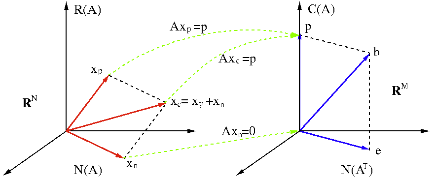
The figure below illustrates a specific case with $M=N=3$ and $R=2$. As ${\bf b}\notin C({\bf A})$, the system can only be approximately solved to find ${\bf Ax}={\bf p}\in C({\bf A})$, which is the projection of ${\bf b}$ onto the column space $C({\bf A})$. The error $\vert\vert{\bf e}\vert\vert=\vert\vert{\bf p}-{\bf b}\vert\vert=\vert\vert{\bf Ax}_p-{\bf b}\vert\vert$ is minimized, ${\bf x}_p$ is the optimal approximation. We will consider ways to obtain this optimal approximation in the following sections.