While solving a linear equation system
 , if
, if  ,
i.e., there are more equations than unknowns, the equation system
may be over-determined with no solution. In this case we can still find
an approximated solution which is optimal in the least squares (LS)
sense, i.e., the LS error defined below is minimized:
,
i.e., there are more equations than unknowns, the equation system
may be over-determined with no solution. In this case we can still find
an approximated solution which is optimal in the least squares (LS)
sense, i.e., the LS error defined below is minimized:
where
 is the residual of an
approximated solution
is the residual of an
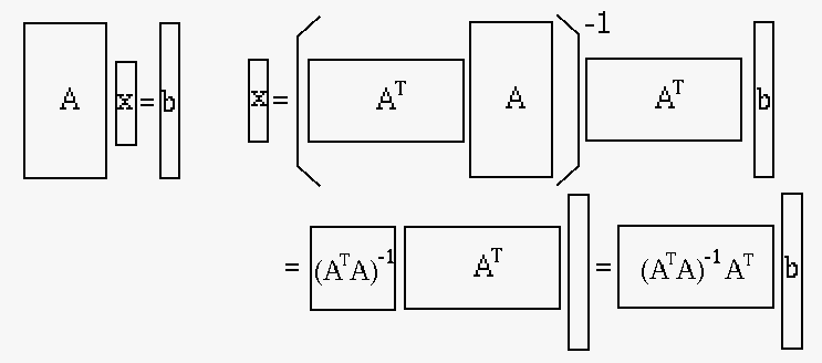
approximated solution  . To find this optimal solution, we
set the derivative of the LS error to zero (see here):
. To find this optimal solution, we
set the derivative of the LS error to zero (see here):
 |
(123) |
and solve this matrix equation to get
 |
(124) |
where
 is the pseudo-inverse
of the non-square matrix
is the pseudo-inverse
of the non-square matrix  .
.
Here we assume the  matrix
 has full rank
with
has full rank
with  and therefore is invertible. However, if
  , matrix
non-invertible. In this case, we can still find san
approximated solution using the
pseudo inverse
of
based on its SVD:
, matrix
non-invertible. In this case, we can still find san
approximated solution using the
pseudo inverse
of
based on its SVD:
 |
(125) |
As we will show below, this solution is optimal in the LS sense.
Moreoever, even if matrix is full rank with , it may still
be nearly singular, with a large condition number
 , i.e.,
some singular values of may be close to zero and the corresponding
singular values of
, i.e.,
some singular values of may be close to zero and the corresponding
singular values of  may be very large. As the result, the
approximated solution may be very large, and prone to noise. Such a system
is said to be ill-conditioned. In this case, to avoid large , we
can impose a penalty term
may be very large. As the result, the
approximated solution may be very large, and prone to noise. Such a system
is said to be ill-conditioned. In this case, to avoid large , we
can impose a penalty term
 in the error function:
 |
(126) |
where  is a parameter that adjusts how tightly the size of is
controlled. Then repeating the process above we get:
is a parameter that adjusts how tightly the size of is
controlled. Then repeating the process above we get:
 |
(127) |
which yields
 |
(128) |
Solving this for we get:
 |
(129) |
Consider the following two linear equation ssytems:
In the first system, there are fewer equations than unknowns
( ), but there exist no solution; in the second system,
there are more equations than unknowns (), but there exist
infinite number of solutions. We therefore see that in general,
if a linear system has no solution, unique solution, or multiple
solutions can not be determined simply by checking if ,
), but there exist no solution; in the second system,
there are more equations than unknowns (), but there exist
infinite number of solutions. We therefore see that in general,
if a linear system has no solution, unique solution, or multiple
solutions can not be determined simply by checking if ,
 , or . This issue of the stucture of the solution set
of a linear equation system
can be fully
addressed by the Fundamental Theorem of Linear Algebra
discussed below.
, or . This issue of the stucture of the solution set
of a linear equation system
can be fully
addressed by the Fundamental Theorem of Linear Algebra
discussed below.
The second system above can be solved by the pseudo inverse methed:
![$\displaystyle {\bf A}=\left[\begin{array}{cc}1&1\\ 2&2\\ 3&3\end{array}\right],...
...=2\left[\begin{array}{ccc}
1 & 2 & 3\\ 2 & 4 & 6 \\ 3 & 6 & 9\end{array}\right]$](img375.svg) |
(130) |
We see that
is a singular and not invertible,
and we cannot get the pseudo inverse by
 .
However, we can still find the pseudo inverse of by
SVD method
.
However, we can still find the pseudo inverse of by
SVD method
 with:
with:
![$\displaystyle {\bf U}=\left[\begin{array}{rrr}
0.2673 & -0.9482 & -0.1719 \\
0...
... V}=\frac{1}{\sqrt{2}}\left[\begin{array}{rr}
1 & 1 \\ 1 &-1 \end{array}\right]$](img378.svg) |
(131) |
and
![$\displaystyle {\bf A}^-={\bf V\Sigma}^-{\bf U}^T
=\left[\begin{array}{rrr}0.0357 & 0.0714 & 0.1071\\
0.0357 & 0.0714 & 0.1071\end{array}\right]$](img379.svg) |
(132) |
Now we can find the solution:
![$\displaystyle {\bf x}={\bf A}^-{b}=\left[\begin{array}{c}1\\ 1\end{array}\right]$](img380.svg) |
(133) |


