In the previous section we obtained the solution of the equation
 together with the bases of the four subspaces
of
together with the bases of the four subspaces
of  based its rref. Here we will consider an alternative
and better way to solve the same equation and find a set of
orthogonal bases that also span the four subspaces, based on the
pseudo-inverse
and
the singular value decomposition (SVD)
of . The solution obtained this
way is optimal in some certain sense as shown below.
based its rref. Here we will consider an alternative
and better way to solve the same equation and find a set of
orthogonal bases that also span the four subspaces, based on the
pseudo-inverse
and
the singular value decomposition (SVD)
of . The solution obtained this
way is optimal in some certain sense as shown below.
Consider the SVD of an  matrix of rank
 :
:
 |
(160) |
where
![$\displaystyle {\bf\Sigma}=\left[\begin{array}{cccccc}\sigma_1&&&&&0\\
&\ddots&...
...&&\sigma_R &&&\\ &&&0&&\\ &&&&\ddots &\\ 0&&&&&0
\end{array}\right]_{M\times N}$](img622.svg) |
(161) |
is an matrix with  non-zero singular values
 of along
the diagonal (starting from the top-left corner), while all other
components are zero, and
of along
the diagonal (starting from the top-left corner), while all other
components are zero, and
![${\bf U}=[{\bf u}_1,\cdots,{\bf u}_M]$](img624.svg) and
and
![${\bf V}=[{\bf v}_1,\cdots,{\bf v}_N]$](img625.svg) are two orthogonal matrices
of dimensions
are two orthogonal matrices
of dimensions  and
and  respectively. The column
vectors
respectively. The column
vectors
 and
and
 ,
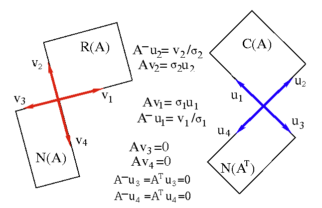
are called the left and right singular vectors of ,
respectively, and they can be used as the orthonormal bases to span
respectively
,
are called the left and right singular vectors of ,
respectively, and they can be used as the orthonormal bases to span
respectively
 and its
subspaces
and its
subspaces
 and
and
 , and
, and
 and its subspaces
and
and its subspaces
and
 .
.
To see this, we rewrite the SVD of as:
Each column vector of can be expressed as a linear
combination of the first columns of  corresponding
to the non-zero singular values:
corresponding
to the non-zero singular values:
 |
(163) |
Taking transpose on both sides of the SVD we also get:
i.e., each row vector of can be expressed as a linear
combination of the first columns of  corresponding
to the non-zero singular values:
corresponding
to the non-zero singular values:
 |
(165) |
We therefore see that the columns of and
corresponding to the non-zero singular values span respectively
the column space
and row space
 :
:
 |
(166) |
and the remaining  columns of and
  columns of
corresponding to the zero singular values span respectively
orthogonal to
, and
orthogonal
to
:
columns of
corresponding to the zero singular values span respectively
orthogonal to
, and
orthogonal
to
:
 |
(167) |
| Subspace |
Definition |
Dimension |
Basis |
 |
column space (image) of |
|
columns of corresponding to non-zero singular values |
 |
left null space of  |
|
columns of corresponding to zero singular values |
 |
row space of (column space of ) |
|
columns of corresponding to non-zero singular values |
 |
null space of |
|
columns of corresponding to zero singular values |
 |
domain of
|
 |
all columns of |
 |
codomain of
|
 |
all columns of |
The SVD method can be used to find the pseudo-inverse of an
matrix of rank
:
 |
(168) |
where both  and
and
![$\displaystyle {\bf\Sigma}^-=\left[\begin{array}{cccccc}1/\sigma_1&&&&&0\\
&\dd...
...1/\sigma_R &&&\\ &&&0&&\\ &&&&\ddots &\\ 0&&&&&0
\end{array}\right]_{N\times M}$](img650.svg) |
(169) |
are  matrices.
Consider the following four cases:
- If
 , then
 ,
,
 .
.
- If
 , then
 (full rank), is a left inverse:
 |
(170) |
However,
 |
(171) |
as the matrix
 with only 1's
along the diagonal is not full rank and unequal to
with only 1's
along the diagonal is not full rank and unequal to
 ,
,
- If
 , the
, the
 (full rank), is a right inverse:
 |
(172) |
However,
 |
(173) |
as the matrix
 with only 1's
along the diagonal is not a full rank identity matrix
with only 1's
along the diagonal is not a full rank identity matrix
 .
.
- If
 , then neither
nor
is full rank, as they only have
non-zeros 1's along the diagonal, therefore is neither
left nor right inverse:
, then neither
nor
is full rank, as they only have
non-zeros 1's along the diagonal, therefore is neither
left nor right inverse:
 |
(174) |
We further note that matrices and are related to each
other by:
 or or |
(175) |
or in vector form:
 |
(176) |
indicating how the individual columns are related.
We see that the last columns
 of
form an orthogonal basis of
; and the last
columns
of
form an orthogonal basis of
; and the last
columns
 of form an orthogonal
basis of
.
of form an orthogonal
basis of
.
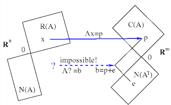
We now show that the optimal solution of the linear system
can be obtained based on the pseudo-inverse
of :
 |
(177) |
Specially, if  , then
, and
, then
, and
 is the unique and exact solution.
In general when
is the unique and exact solution.
In general when  or
, the solution may not
exist, or it may not be unique, but
or
, the solution may not
exist, or it may not be unique, but
 is still an
optimal solution in two ways, from the perspective of both the
domain and codomain of the linear mapping
is still an
optimal solution in two ways, from the perspective of both the
domain and codomain of the linear mapping  , as shown below.
- In domain
 :
:
Pre-multiplying
 on both sides of the
pseudo-inverse solution
on both sides of the
pseudo-inverse solution
 given above,
we get:
given above,
we get:
![$\displaystyle {\bf V}^T{\bf x}_{svd}
=[{\bf v}_1,\cdots,{\bf v}_N]^T{\bf x}_{sv...
...f\Sigma}^-{\bf U}^T{\bf b}
={\bf\Sigma}^-[{\bf u}_1,\cdots,{\bf u}_M]^T{\bf b},$](img677.svg) |
(178) |
or in component form:
![$\displaystyle \left[\begin{array}{c}{\bf v}_1^T{\bf x}_{svd}\\ \vdots\\
{\bf v...
...ma_1\\ \vdots\\
{\bf u}_R^T{\bf b}/\sigma_R\\ 0\\ \vdots\\ 0\end{array}\right]$](img678.svg) |
(179) |
- The first components
 are the projection of
onto
spanned by
are the projection of
onto
spanned by
 corresponding to the non-zero
singular values;
corresponding to the non-zero
singular values;
- The last components
 are the projection
of
onto
spanned by
are the projection
of
onto
spanned by
 corresponding to the zero
singular values.
corresponding to the zero
singular values.
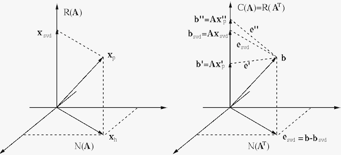
We see that
 is entirely in the row space,
containing no homogeneous component in
, i.e.,
has the minimum norm (closest to the origin) compared to any other possible
solution
is entirely in the row space,
containing no homogeneous component in
, i.e.,
has the minimum norm (closest to the origin) compared to any other possible
solution  , such as those found previously based on the rref
of , containing a non-zero homogeneous component
, such as those found previously based on the rref
of , containing a non-zero homogeneous component
 :
:
 |
(180) |
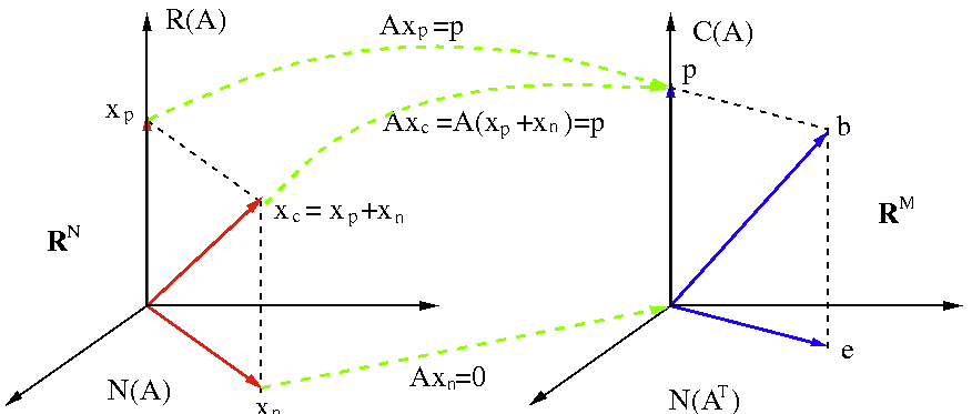
As
 ,
is the
projection of any such solution onto
. The
complete solution can be found as
,
is the
projection of any such solution onto
. The
complete solution can be found as
 |
(181) |
for any set of coefficients  .
.
- In codomain
 :
:
We now consider the result
 produced
by the pseudo-inverse solution
, which, as a linear
combination of the columns of , is in its column space
:
produced
by the pseudo-inverse solution
, which, as a linear
combination of the columns of , is in its column space
:
 |
(182) |
Pre-multiplying
 on both sides we get:
 |
(183) |
or in component form:
![$\displaystyle \left[\begin{array}{c}{\bf u}_1^T{\bf b}_{svd}\\ \vdots\\
{\bf u...
...u}_1^T{\bf b}\\ \vdots\\
{\bf u}_R^T{\bf b}\\ 0\\ \vdots\\ 0\end{array}\right]$](img691.svg) |
(184) |
We see that
 is entirely in the column
space. If
is entirely in the column
space. If
 , then
 is an
exact solution. But if
is an
exact solution. But if
 , then
 and
is not an exact solution.
But as
is the projection of
and
is not an exact solution.
But as
is the projection of  onto
, the error
onto
, the error
 is minimized in
comparison to any other possible
is minimized in
comparison to any other possible

 |
(185) |
We therefore see that
is the optimal solution.
Summarizing the two aspects above, we see that the pseudo-inverse
solution
is optimal in the sense that both its
norm
 and its error
 are minimized.
- If the solution
is not unique because
 , then the complete solution can be
found by adding the entire null space to it:
, then the complete solution can be
found by adding the entire null space to it:
 .
.
- If no solution exists because
,
then
is the optimal approximate solution with
minimum error.
Example: Given the same system considered in previous examples
we will now solve it using the pseudo-inverse method. We first find SVD of
in terms of the following matrices:
The particular solution of the system
 with
with
![${\bf b}=[3,\;2,\;4]^T\in C({\bf A})$](img713.svg) is
is
which is in
spanned by the first  columns
 and
and  , perpendicular to
spanned
by the last
, perpendicular to
spanned
by the last  columns
  and
and  . Note that
this solution
. Note that
this solution
![${\bf x}_{svd}=[0.1,\;0.2,\;0.3,\;0.4]^T$](img721.svg) is actually
the first component
is actually
the first component
 of the particular
solution
of the particular
solution
![${\bf x}_p=[-1,\,2,\,0,\,0]$](img723.svg) found in the previous section
by Gauss-Jordan elimination, which is not in
. Adding the
null space to the particular solution, we get the complete solution:
If the right-hand side is replaced by
found in the previous section
by Gauss-Jordan elimination, which is not in
. Adding the
null space to the particular solution, we get the complete solution:
If the right-hand side is replaced by
![${\bf b}=[1,\;3,\;5]^T\notin C({\bf A})$](img599.svg) , no solution exists. However, we can still find the
pseudo-inverse solution as the optimal approximate solution:
which is the same as the solution for
, no solution exists. However, we can still find the
pseudo-inverse solution as the optimal approximate solution:
which is the same as the solution for
![${\bf b}=[3,\;2,\;4]^T$](img726.svg) ,
indicating
,
indicating
![$[3,\;2,\;4]^T$](img727.svg) happens to be the projection of
happens to be the projection of
![$[1,\;3,\;5]^T$](img728.svg) onto
spanned by
onto
spanned by  and
and
 . The result produced by
is
. The result produced by
is
 is the projection of
onto
, with a minimum error distance
is the projection of
onto
, with a minimum error distance
 , indicating
is the optimal approximate solution.
, indicating
is the optimal approximate solution.
Homework 3:
- Use Matlab function
svd(A) to carry out the SVD of the coefficient
matrix of the linear system in Homework 2 problem 3,
Find , ,
 . Verify that and
are orthogonal, i.e.,
. Verify that and
are orthogonal, i.e.,
 and
and
 .
.
- Obtain
 , i.e, find the transpose of
and then replace each singular value by its reciprocal, verify that
, i.e, find the transpose of
and then replace each singular value by its reciprocal, verify that
 and
and
 .
Then find the pseudo-inverse
.
Then find the pseudo-inverse
 .
.
- Use Matlab function
pinv(A) to find the pseudo-inverse
and . Compare them to what you obtained
in the previous part.
- Identify the bases of the four subspaces
,
,
 , and
based on and
. Verify that these bases and those you found previously (problem
3 of Homework 2) span the same spaces, i.e., the basis vectors of one basis
can be written as a linear combination of those of the other, for each of
the four subspaces.
, and
based on and
. Verify that these bases and those you found previously (problem
3 of Homework 2) span the same spaces, i.e., the basis vectors of one basis
can be written as a linear combination of those of the other, for each of
the four subspaces.
- Use the pseudo-inverse found above to solve
the system
. Find the two particular solutions
 and
and
 corresponding to two different right-hand
side
corresponding to two different right-hand
side
![${\bf b}_1=[1,\;2,\;3]^T$](img742.svg) and
and
![${\bf b}_2=[2,\;3,\;2]^T$](img743.svg) .
.
- How are the two results
and
related to
each other? Give your explanation. Why can't you find a solution when
![${\bf b}=[2,\;3,\;2]^T$](img744.svg) but SVD method can?
but SVD method can?
- Verify that
 . Also find the error (or
residual)
. Also find the error (or
residual)
 for each of the two results
above. Verify that
for each of the two results
above. Verify that
 , if
, if
 .
.
- In Homework 2 you used row reduction method to solve the system
 and you should have found a particular solution
![${\bf x}_1=[5,\;2,\;0,\;0,\;]^T$](img750.svg) . Also it is obvious to see that another
solution is
. Also it is obvious to see that another
solution is
![${\bf x}_2=[0,\;0,\;0,\;1]^T$](img751.svg) . Show that the projection of
these solutions onto
spanned by the first two columns of
is the same as the particular solution found by
the SVD method.
. Show that the projection of
these solutions onto
spanned by the first two columns of
is the same as the particular solution found by
the SVD method.
Answer
- Show that
is the projection of
onto
, the 2-D subspace spanned by
the first two columns of . Can you also show that it is the
projection of onto
spanned by the basis you obtained
in Homework 2 (not necessarily orthogonal)?
Answer
- Give an expression of the null space
, and then write the
complete solution in form of
 . Verify any
complete solution so generated satisfies
. Verify any
complete solution so generated satisfies
 .
.


![$\displaystyle [{\bf c}_1,\cdots,{\bf c}_N]={\bf U\Sigma V}^T$](img631.svg)
![$\displaystyle [{\bf u}_1,\cdots\cdots\cdots,{\bf u}_M]
\left[\begin{array}{cccc...
...array}{c}{\bf v}_1^T\\ \vdots\\ \vdots\\ \vdots\\ {\bf v}_N^T\end{array}\right]$](img632.svg)
![$\displaystyle \sum_{k=1}^R \sigma_k\;\left({\bf u}_k{\bf v}_k^T\right)
=\sum_{k...
...gma_kv_{1k})\;{\bf u}_k,\cdots,
\sum_{k=1}^R (\sigma_kv_{Nk})\;{\bf u}_k\right]$](img633.svg)

![$\displaystyle [{\bf r}_1,\cdots,{\bf r}_M]
={\bf V\Sigma}^T{\bf U}^T$](img637.svg)
![$\displaystyle \sum_{k=1}^R \sigma_k\;\left({\bf v}_k{\bf u}_k^T\right)
=\sum_{k...
...ku_{1k})\;{\bf v}_k,\;\cdots,\;
\sum_{k=1}^R (\sigma_ku_{Mk})\;{\bf v}_k\right]$](img638.svg)
 ,
i.e.,
,
i.e.,
 and
and  corresponding
to the non-zero singular values.
corresponding
to the non-zero singular values.
 are the projection
of
are the projection
of
 corresponding to the zero
singular values.
corresponding to the zero
singular values.
![$\displaystyle {\bf A}{\bf x}=\left[\begin{array}{rccc}1&2&3&4\\ 4&3&2&1\\ -2&1&...
... x_3\\ x_4\end{array}\right]
=\left[\begin{array}{r}3\\ 2\\ 4\end{array}\right]$](img706.svg)
![$\displaystyle {\bf U}=[{\bf u}_1,\;{\bf u}_2,\;{\bf u}_3]
=\left[\begin{array}{...
...817 \\
-0.267 & -0.873 & -0.408 \\
-0.802 & 0.436 & -0.408 \end{array}\right]$](img707.svg)
![$\displaystyle {\bf V}=[{\bf v}_1,\;{\bf v}_2,\;{\bf v}_3,\;{\bf v}_4]
=\left[\b...
... -0.120 & 0.472 & 0.691 \\
-0.802 & 0.239 & -0.049 & -0.546 \end{array}\right]$](img708.svg)
![$\displaystyle {\bf\Sigma}=\left[\begin{array}{cccc}
10.0 & 0 & 0 & 0 \\
0 & 5....
...c}
0.1 & 0 & 0 \\
0 & 0.183 & 0 \\
0 & 0 & 0 \\
0 & 0 & 0 \end{array}\right]$](img709.svg)

![$\displaystyle \left[\begin{array}{rrrr}
0.000 & -0.837 & 0.374 & -0.400 \\
-0....
....802 \\
-0.218 & -0.873 & 0.436 \\
0.817 & -0.408 & -0.408 \end{array}\right]$](img711.svg)
![$\displaystyle \left[\begin{array}{rrr}
0.033 & 0.133 & -0.067 \\
0.033 & 0.083 & -0.017 \\
0.033 & 0.033 & 0.033 \\
0.033 & -0.017 & 0.083 \end{array}\right]$](img712.svg)

![$\displaystyle {\bf A}^-{\bf b}=\left[\begin{array}{rrr}
0.033 & 0.133 & -0.067 ...
...nd{array}\right]
=\left[\begin{array}{r}0.1\\ 0.2\\ 0.3\\ 0.4\end{array}\right]$](img715.svg)
![$\displaystyle -0.535\left[\begin{array}{r}0.000\\ -0.267\\ -0.535\\ -0.802\end{...
...r}-0.837\\ -0.478\\ -0.120\\ 0.239\end{array}\right]
=c_1{\bf v}_1+c_2{\bf v}_2$](img716.svg)
![$\displaystyle {\bf x}_c={\bf x}_{svd}+N({\bf A})={\bf x}_p+c_1{\bf v}_3+c_2{\bf...
...t]
+c_2 \left[\begin{array}{r}-0.400\\ 0.255\\ 0.691\\ -0.546\end{array}\right]$](img724.svg)
![$\displaystyle {\bf x}_{svd}={\bf A}^-{\bf b}=\left[\begin{array}{rrr}
0.033 & 0...
...nd{array}\right]
=\left[\begin{array}{r}0.1\\ 0.2\\ 0.3\\ 0.4\end{array}\right]$](img725.svg)
![$\displaystyle {\bf A}=\left[\begin{array}{rrrr}-1 & 3 & 4 & 1\\
2 & -4 & 3 & 2\\ 1 & -1 & 7 & 3\end{array}\right]$](img733.svg)


![$\displaystyle c_1{\bf u}_1+c_2{\bf u}_2=[1,\;2,\;3]^T={\bf b}_1$](img757.svg)