Next: Perceptron Learning
Up: Introduction to Neural Networks
Previous: Hebb's Learning
Hopfield network
(Hopfield 1982)
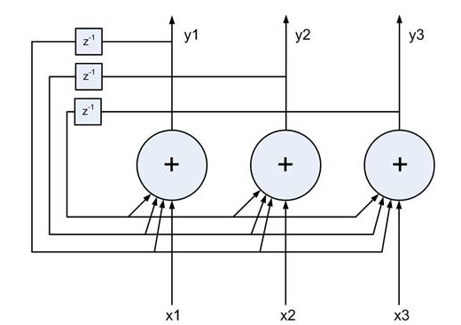
is recurrent network composed of a set of  nodes and behaves as an
auto-associator (content addressable memory) with a set of
nodes and behaves as an
auto-associator (content addressable memory) with a set of  patterns
 stored in it. The network is first trained
in the fashion similar to that of the Hebbian learning, and then used as an
auto-associator. When the incomplete or noisy version of one of the stored
patterns is presented as the input, the complete pattern will be generated as
the output after some iterative computation.
stored in it. The network is first trained
in the fashion similar to that of the Hebbian learning, and then used as an
auto-associator. When the incomplete or noisy version of one of the stored
patterns is presented as the input, the complete pattern will be generated as
the output after some iterative computation.
Presented with a new input pattern (e.g., noisy, incomplete version of
some pre-stored pattern)  :
:
the network responds by iteratively updating its output
until finally convergence is reached when one of the stored patterns which
most closely resembles  is produced as the output.
The training process
The training process is essentially the same as the Hebbian learning, except
here the two associated patterns in each pair are the same (self-association),
i.e.,
 , and the input and output patterns all have the
same dimension
, and the input and output patterns all have the
same dimension  .
.
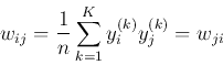
After the network is trained by Hebbian learning its weight matrix is obtained
as the sum of the outer-products of the patterns to be stored:
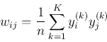
the weight connecting node i and node j is
And we assume no self-connection exists
After the weight matrix  is obtained by the training process, the
network can be used to recognize any input pattern representing some noisy
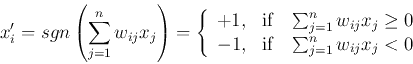
and incomplete version of one of those pre-stored patterns. When an input
pattern is presented to the input nodes, the outputs nodes are
updated iteratively and asynchronously. Only one of the nodes
randomly selected is updated at a time:
is obtained by the training process, the
network can be used to recognize any input pattern representing some noisy
and incomplete version of one of those pre-stored patterns. When an input
pattern is presented to the input nodes, the outputs nodes are
updated iteratively and asynchronously. Only one of the nodes
randomly selected is updated at a time:
where  represents the new output of the ith node while
  represents the old one during the iteration. We will now show that the iteration
will always converge to produce one of the stored patterns as the output.
represents the old one during the iteration. We will now show that the iteration
will always converge to produce one of the stored patterns as the output.
Energy function
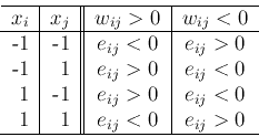
We define the energy associated with a pair of nodes i and j as
and the interaction between these two nodes can be summarized by this table
Two observations:
- Whenever the two nodes i and j are reinforcing each other's state, the
energy
 is negative. For example, in the first and last rows when
 ,
,  will help keep
  to stay at the same state
  ,
and the energy
,
and the energy  is negative. Also in the two middle rows when
 , will help keep to stay at the same state
  ,
and the energy is negative.
,
and the energy is negative.
- Whenever the two nodes i and j are trying to change each other's state,
the energy is positive. For example, in the first and last rows when
, will tend to reverse from its previous state
to , and the energy
 is positive. Also in the two
middle rows when , will tend to reverse from its
previous state to , and the energy is positive.
is positive. Also in the two
middle rows when , will tend to reverse from its
previous state to , and the energy is positive.
In other words, low energy level of corresponds to a stable interaction
between  and , and high energy level corresponds to an unstable
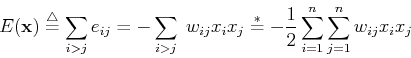
interaction. We next define the total energy function
and , and high energy level corresponds to an unstable
interaction. We next define the total energy function  of
all nodes in the network as the sum of all the pair-wise energies:
of
all nodes in the network as the sum of all the pair-wise energies:
Note that the last equation is due to  . Again, lower energy
function level corresponds to more stable condition of the network, and vice
versa.
. Again, lower energy
function level corresponds to more stable condition of the network, and vice
versa.
The iteration and convergence
Now we show that the total energy always decreases whenever the
state of any node changes. Assume  has just been updated, i.e.,
 (
( but
but  ), while all others remain the same
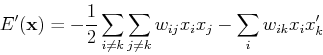
 . The energy before changes state is
and the energy after changes state is
The energy difference is
Consider two cases:
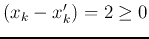
- Case 1: if
 but
but
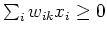 , then
  , we
have
, we
have
 and
and
 .
.
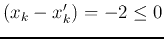
- Case 2: if
 but
but
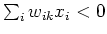 , then
  , we
have
, we
have
 and
.
and
.
As
 is always true throughout the iteration,
and the magnitude of is finite, we conclude that the energy
function will eventually reach one of the minima of the
``energy landscape'' and, therefore, the iteration will always converge.
is always true throughout the iteration,
and the magnitude of is finite, we conclude that the energy
function will eventually reach one of the minima of the
``energy landscape'' and, therefore, the iteration will always converge.
Retrieval of stored patterns
Here we show the pre-stored patterns correspond to the minima of the
energy function. First recall the weights of the network are obtained by
Hebbian learning:
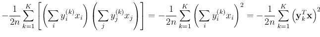
The energy function can now be written as
If is different from any of the stored patterns, all terms of the
summation will contribute to the sum only moderately. However, if is
the same as any of the stored patterns, their inner product reaches maximum,
and thus causing the total energy to be minimized to reach one of the minima.
In other words, the patterns stored in the net correspond to the local minima
of the energy function. i.e., these patterns become attractors.
Note that it is possible to have other local minima, called spurious
states, which do not represent any of the stored patterns, i.e., the
associative memory is not perfect.
Next: Perceptron Learning
Up: Introduction to Neural Networks
Previous: Hebb's Learning
Ruye Wang
2015-08-13
![\begin{displaymath}
{\bf W}_{n\times n}=\frac{1}{n}\sum_{k=1}^K {\bf y}_k {\bf ...
...n^{(k)} \end{array} \right]
[ y_1^{(k)}, \cdots, y_n^{(k)} ]
\end{displaymath}](img94.png)

![$\displaystyle -\frac{1}{2}\sum_{i=1}^{n} \sum_{j=1}^{n} w_{ij} x_i x_j =
-\frac...
...\frac{1}{2n}\sum_{k=1}^K \left[\sum_i \sum_j y_i^{(k)} x_i y_j^{(k)} x_j\right]$](img135.png)