Next: Appendix A: Kullback-Leibler (KL)
Up: MCMC and EM Algorithms
Previous: Expectation Maximization (EM)
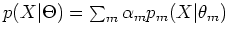
Assume  random samples
 are drawn from a mixture
distribution
are drawn from a mixture
distribution
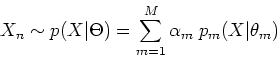
where  is the mth distribution component parameterized by
 , and
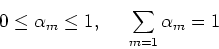
, and  is the mixing coeficient or prior probability
of each mixture component satisfying
is the mixing coeficient or prior probability
of each mixture component satisfying
The parameters are
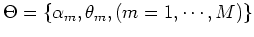 .
As
are independent, their joint distribution is
.
As
are independent, their joint distribution is
and the log-likelihood of the parameters is
Finding a  that maximizes this log-likelihood is not easy. To
make the problem easier, now assume some hidden or latent ramdom variables
that maximizes this log-likelihood is not easy. To
make the problem easier, now assume some hidden or latent ramdom variables
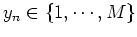
![$Y=[y_1,\cdots,y_N]^T$](img157.png) , where
, where
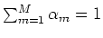
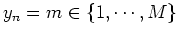 if the nth sample
 is generated by the mth component
 of the mixture
distribution. Now the log-likelihood can be written in terms of both
of the mixture
distribution. Now the log-likelihood can be written in terms of both  and
and  :
:
The last equal sign is due to the definition of  , i.e., is known
to be generated by the th distribution component
, i.e., is known
to be generated by the th distribution component  , therefore
all other terms in the summation
, therefore
all other terms in the summation
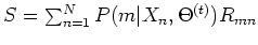
 can be dropped. The expectation of the log-likelihood with respect to is
![\begin{displaymath}Q(\Theta,\Theta^{(t)})=E_Y \;log[L(\Theta\vert X,Y)]
=\sum_Y log[L(\Theta\vert X,Y)]\; p(Y\vert X,\Theta^{(t)}) \end{displaymath}](img167.png)
But as any
 can only take one of these
  integers,
the expectation above can be written as
integers,
the expectation above can be written as
The two terms can be maximized separately as and
are not related.
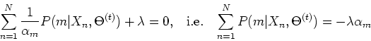
- Find
To find that maximize the first term, we solve the following
where  is the Lagrange multiplier to impose the constraint
 in the opptimizatioin. Solving this equation,
we get:
in the opptimizatioin. Solving this equation,
we get:
Summing both sides over 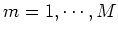 , we get
which yields
and
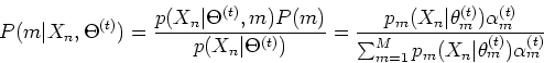
These probabilities
 can be found by Bayes's rule:
where
on the left is the probability for a given sample
to be from the  th component distribution,
 is
the probability of given that it is from the th component distribution,
is
the probability of given that it is from the th component distribution,
 is the a priori probability of the th component, which is the
same as the coeficient
is the a priori probability of the th component, which is the
same as the coeficient
 for that component. Given the current
estimation of the parameters
for that component. Given the current
estimation of the parameters
 of the specific distributions, all variables on the
right-hand side are available and the conditional probabilities of the
hidden variables can be obtained.
of the specific distributions, all variables on the
right-hand side are available and the conditional probabilities of the
hidden variables can be obtained.
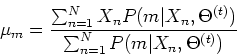
- Find
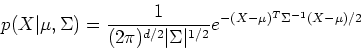
Given a specific distribution function, e.g., a Gaussian distribution
where  and
and  are the mean vector and the covariance matrix
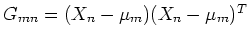
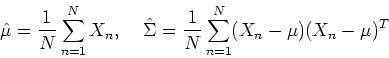
which can be estimated by
are the mean vector and the covariance matrix
which can be estimated by
we can proceed to find the parameters
 that
maximize the second term of the log-likelihood function above by solving
that
maximize the second term of the log-likelihood function above by solving
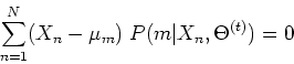
Taking the log inside and dropping the constants, we get
First consider taking derivative with respect to  of ,
we get
of ,
we get
i.e.,
which can be solved for to get
Next consider taking derivative with respect to  of .
We first rearrange the log-likelihood function above to get
of .
We first rearrange the log-likelihood function above to get
where
 . Then taking the derivative with
respect to
. Then taking the derivative with
respect to  and setting it to zero, we get (see Appendix B):
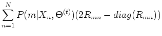
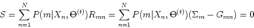
where
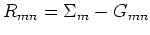 ,
,
 .
This result implies
.
This result implies  , i.e.,
This leads to
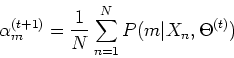
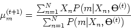
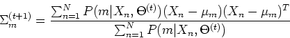
The results obtained above can be summarized as below:
Although the above derivation seems tedius, but the final results all
make sense intuitively: the coeficient for the th component
distribution is the average of the posterior probabilities
for the samples to be from the mth component
distribution, and the estimated mean vector is the average of the
samples , and the estimated covariance matrix is the
average of the difference between and squared, both weighted by
the posterior probability
that a given is
from the mth component distribution  . Also note that both the E
and M steps are simultaneously carried out by these three iterative
equations, from some arbitrary initial guesses of these parameters.
. Also note that both the E
and M steps are simultaneously carried out by these three iterative
equations, from some arbitrary initial guesses of these parameters.
Next: Appendix A: Kullback-Leibler (KL)
Up: MCMC and EM Algorithms
Previous: Expectation Maximization (EM)
Ruye Wang
2006-10-11
![$\displaystyle log(p(X\vert\Theta)=log[\prod_{n=1}^N p(X_n\vert\Theta)]
=\sum_{n=1}^N log\; p(X_n\vert\Theta)$](img154.png)
![$\displaystyle \sum_{n=1}^N log[ \sum_{m=1}^M \alpha_m
p_m(X_n\vert\theta_m)]$](img155.png)
![$\displaystyle log[p(X,Y\vert\Theta)]=log[\prod_{n=1}^N p(X_n,Y\vert\Theta)]
=\sum_{n=1}^N log\; [p(X_n\vert Y,\Theta)p(Y)]$](img162.png)
![$\displaystyle \sum_{n=1}^N log\; [\alpha_{y_n} p_{y_n}(X_n\vert\theta_{y_n})]$](img163.png)
![$\displaystyle E_Y \;log[L(\Theta\vert X,Y)]
=\sum_{m=1}^M [\sum_{n=1}^N log\; [\alpha_{m} p_{m}(X_n\vert\theta_{m})] ]
P(m\vert X_n,\Theta^{(t)})$](img171.png)
![$\displaystyle \sum_{m=1}^M \sum_{n=1}^N log\;(\alpha_m)\;P(m\vert X_n,\Theta^{(...
...m_{m=1}^M \sum_{n=1}^N log\;[p_{m}(X_n\vert\theta_m)]P(m\vert X_n,\Theta^{(t)})$](img172.png)
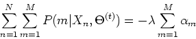
![\begin{displaymath}\frac{\partial}{\partial \alpha_m}\left[ \sum_{m=1}^M \sum_{n...
... X_n,\Theta^{(t)}) +\lambda(\sum_{m=1}^M \alpha_m-1) \right]=0 \end{displaymath}](img173.png)
![$\displaystyle \frac{\partial}{\partial \theta_m} \left[
\sum_{m=1}^M \sum_{n=1}^N log\;[p_m(X_n\vert\theta_m)]P(m\vert X_n,\Theta^{(t)}) \right]$](img192.png)
![$\displaystyle \frac{\partial}{\partial \theta_m} \left[ \sum_{m=1}^M \sum_{n=1}...
..._n-\mu_m)^T\Sigma_m^{-1}(X_n-\mu_m)/2}
]
\;P(m\vert X_n,\Theta^{(t)}) \right]=0$](img193.png)
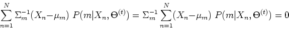
![\begin{displaymath}
\frac{\partial}{\partial \theta_m} \left[ \sum_{m=1}^M \sum_...
...igma_m^{-1}(X_n-\mu_m))
\;P(m\vert X_n,\Theta^{(t)}) \right]=0
\end{displaymath}](img194.png)
![$\displaystyle \sum_{m=1}^M \left[ \sum_{n=1}^N [
log \vert\Sigma_m^{-1}\vert-(X_n-\mu_m)^T\Sigma_m^{-1}(X_n-\mu_m)]
\;P(m\vert X_n,\Theta^{(t)})\right]$](img200.png)
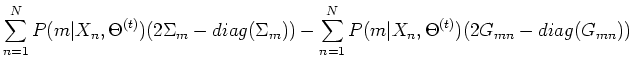
![$\displaystyle \sum_{m=1}^M\left[
log \vert\Sigma_m^{-1}\vert \sum_{n=1}^N \;P(m...
...N \;P(m\vert X_n,\Theta^{(t)})
tr[\Sigma_m^{-1}(X_n-\mu_m)(X_n-\mu_m)^T]\right]$](img201.png)
![$\displaystyle \sum_{m=1}^M\left[log \vert\Sigma_m^{-1}\vert \sum_{n=1}^N \;P(m\...
...t)})
-\sum_{n=1}^N \;P(m\vert X_n,\Theta^{(t)})
tr[\Sigma_m^{-1} G_{mn}]\right]$](img202.png)