Next: EM Method for Parameter
Up: MCMC and EM Algorithms
Previous: Metropolis-Hastings algorithm
Assume the a priori distribution of the parameters is
 and the distribution of the data is
  , then
the joint probability of both the data and parameters is
, then
the joint probability of both the data and parameters is
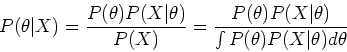
The posterior distribution of the model parameters can be
obtained according to Bayesian theorem:
where
 is the likelihood function
of the parameters
is the likelihood function
of the parameters  , given the observed data
  .
The goal of maximum-likelihood estimation is to find that
maximizes the likelihood
.
The goal of maximum-likelihood estimation is to find that
maximizes the likelihood  :
:
The expectation-maximization (EM) algorithm is a method for finding
maximum likelihood estimates of the parameters of a
probabilistic model, based on unobserved or hidden variables  ,
as well as the observed variables .
,
as well as the observed variables .
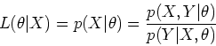
Let  be the complete data containing both the observed (but
incomplete) data and the missing or hidden data , the the
complete-data likelihood of the parameters is
be the complete data containing both the observed (but
incomplete) data and the missing or hidden data , the the
complete-data likelihood of the parameters is
which is a random variable, since the missing data is unknown,
assumed to be random with some distribution, and according to Bayes
rule, the incomplete-data likelihood is
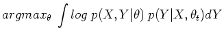
The EM algorithm attempts to find the value of which
maximizes  given the observed , by making use of
the associated family
given the observed , by making use of
the associated family
 [Dempster et al., 1977].
EM alternates between the following two steps:
[Dempster et al., 1977].
EM alternates between the following two steps:
In the E step, the first argument of
 represents the parameter to be optimized to maximize the likelihood,
while the second argument
represents the parameter to be optimized to maximize the likelihood,
while the second argument  represents the parameters used to
evaluate the expectation. In the M step,
represents the parameters used to
evaluate the expectation. In the M step,  is the value
that maximizes (M) the conditional expectation (E) of the complete data
log-likelihood given the observed variables under the previous
parameter value . The parameters found on
the M step are then used to begin another E step, and the process is
repeated.
is the value
that maximizes (M) the conditional expectation (E) of the complete data
log-likelihood given the observed variables under the previous
parameter value . The parameters found on
the M step are then used to begin another E step, and the process is
repeated.
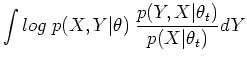
Also note that the last equal sign is due to the fact that the denominator
 is not a function and is therefore independent of the
parameters . In other words, the
is not a function and is therefore independent of the
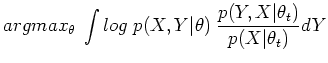
parameters . In other words, the  function in the E step
can also be written as
function in the E step
can also be written as
Theorem: The procedure in M step above quarantees that
with equality iff
 .
.
Proof:
As
 , we have
where
 is defined as
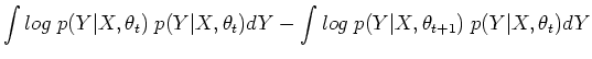
Now we get:
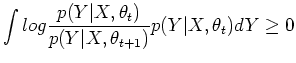
as the first term is greater than or equal to 0 due to the M step of the
algorithm, and we can show the second term is also greater than or equal to 0:
The last expression is Kullback-Leibler information divergence
(KL divergence), which is always non-negative, or zero if
Example: Assume observed variable  and hidden variablle
  are independently and identically generated by an exponential
distribution
are independently and identically generated by an exponential
distribution
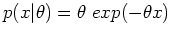 (
( ):
):
Then the joint distribution of  and is
and the log likelihood is
As and are independent, the conditional probability of is
The E step: compute
:
The M step: maximize
:
which can be solved to yield the iteration formula:
This iteration will always converge to
 , independent of
the initial value
, independent of
the initial value  . In fact, for any value of the observed sample
, the iteration will converge to
. In fact, for any value of the observed sample
, the iteration will converge to  , agreeing with the observed
value
, agreeing with the observed
value  .
.
Next: EM Method for Parameter
Up: MCMC and EM Algorithms
Previous: Metropolis-Hastings algorithm
Ruye Wang
2006-10-11
![$\displaystyle E_Y\;[ log\;p(X,Y\vert\theta)\vert X,\theta_t]
=\int log\;p(X,Y\vert\theta) \;p(Y\vert X,\theta_t) dY$](img99.png)