Markov Chain Monte Carlo (MCMC)

Monte Carlo methods can solve these general problems:

• draw random variables from a probability density function $p(X)$
• estimate integral
  
  $$\int f(X) p(X) dX=E_p \; f(X)$$
  
  

Monte Carlo methods can be used to evaluate the integrations for $E[f(X)]$ in Baysian inference, by drawing samples $\{X_t, t=1,\cdots, n\}$ from $p(X)$ and then approximating

$$E[f(X)]\approx \frac{1}{n}\sum_{t=1}^n f(X_t)$$

This is referred to as Monte Carlo integration.

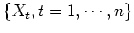
A Markov Chain is a sequence of random variables $\{X_0,X_1,\cdots\}$ generated by a Markov process. At each time $t \ge 0$, the next state $X_{t+1}$ is sampled from a distribution called transition kernel $P(X_{t+1}\vert X_t) \stackrel{\triangle}{=} Prob(X_t \rightarrow X_{t+1})$. By definition, the next state $X_{t+1}$ of a Markov process only depends on the current state $X_t$, but is independent of all previous states $X_0, X_1, \cdots, X_{t-1}$ (limited horizon):

$$P(X_{t+1}\vert X_0, X_1, \cdots X_t) = P(X_{t+1}\vert X_t)$$

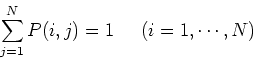
Let $\{s_i, (i=1,\cdots,N) \}$ be the $N$ possible states of the Markov chain. We define

• $p_i(t)\stackrel{\triangle}{=}Prob(X_t=s_i)$ as the ith component of the $N\times 1$ distribution vector of the t-th state ${\bf p}=[p_1(t),\cdots,p_N(t)]^T$,
• $P(i,j)\stackrel{\triangle}{=}Prob(j\rightarrow i)$ as the component in the ith row, jth column of the $N\times N$ transition probability matrix ${\bf P}$. As any current state value $X_t=s_j$ has to lead to one of the $N$ values $X_{t+1}=s_i$ $(i=1,\cdots,N)$ for the next state, we have
  
  $$\sum_{j=1}^N P(i,j)=1 \;\;\;\;\;(i=1,\cdots,N)$$
  
  
  i.e., each column of ${\bf P}$ has to sum to 1.

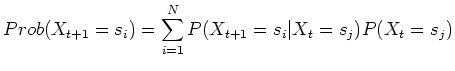
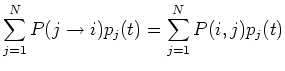
Then the following Chapman-Kolomogrov equation gives the probability of the next state taking a specific value $s_i$:

$$p_i(t+1) = Prob(X_{t+1}=s_i)=\sum_{i=1}^N P(X_{t+1}=s_i\vert X_t=s_j)P(X_t=s_j)$$

$$= \sum_{j=1}^N P(j\rightarrow i) p_j(t)=\sum_{j=1}^N P(i,j) p_j(t)$$

We represent both distributions at stage $t$ and $t+1$ column vectors:

$${\bf p}(t)=[p_1(t),\cdots,p_N(t)]^T, \;\;\;\; {\bf p}(t+1)=[p_1(t+1),\cdots,p_N(t+1)]^T$$

then the Chapman-Kolomogrov equation can be expressed in matrix form:

$${\bf p}(t+1)={\bf P} \; {\bf p}(t)$$

This state transition can be recursively extended until reaching the initial state ${\bf p}(0)$:

$${\bf p}(t+1)={\bf P} \; {\bf p}(t)={\bf P}{\bf P}\;{\bf p}(t-1) = \cdots = {\bf P}^{t+1} \; {\bf p}(0)$$

If the Markov chain is irreducible and aperiodic, the distribution ${\bf p}(t)$ may reach a stationary distribution ${\bf p}^*$ after a large number of transitions, independent of the initial distribution ${\bf p}^*(t)$. Any further transition will not change the distribution any more:

$${\bf p}^*={\bf P}\;{\bf p}^*$$

In other words, the stationary distribution ${\bf p}^*$ is the eigenvector of the transition matrix ${\bf P}$ corresonding to the eigenvalue $\lambda=1$.

A sufficient condition for a unique stationary distribution is that the detailed balance equation holds:

$$P(i\rightarrow j) p_i^*=P(j\rightarrow i) p_j^*$$

under this condition the chain is reversible, and the ith element of vector ${\bf P} {\bf p}$ is

$$({\bf P} {\bf p})_i=\sum_k P(k\rightarrow i) p_k =\sum_k P(i\rightarrow k) p_i=p_i\sum_k P(i\rightarrow k)=p_i$$

(last equal sign due to $\sum_k P(i \rightarrow k)=1$), i.e., ${\bf p}$ is stationary. This condition guarantees stationary distribution from the beginning of the chain, and is not a necessary condition as the chain can also become stationary gradually.