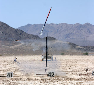
Modeling and Measuring the Dynamics of Rocket Flight

Objective
By the end of the laboratory the student will:
- Develop a numerical model of rocket flight from lift-off to apogee and use that model and data they have collected to predict their rocket's flight.
- Compare their code results with results from commercial rocket codes from lift-off to apogee.
- Develop numerical routines to analyze ther flight data for comparison with their models.
Notice - The Thrust Curves from 2009 haven't been posted yet. Look for updates just before lab starts.
Section 1 – Numerical Methods
- Develop and implement a numerical model to integrate the equations of motion for the rocket flight from liftoff to apogee. Input variables should include time step; sidewind magnitude; parameters associated with the different rockets available for launch; and parameters associated with the available motors (you may use thrust curve data from the Class Thrust Curves or the thrust curves included with the motors. The outputs of the model should include global position, velocity, and acceleration predictions, as well as maximum altitude reached by the rocket. How much of a difference does drag make in the model? You can double check your model with the solutions to Section 5 of the Wind Tunnel lab and Section 4 of the Static Motor Test lab.
- Test the model for the medium rocket, with a coefficient of drag of 0.75, a constant sidewind magnitude of 3 mph, using the first G79W-M motor from 3/8/2008, and time steps of 0.5, 0.05, and 0.005 seconds. Plot the trajectory and predict the maximum altitude of the rocket. You may want to look at the Rocksim model to get dimensions, mass, center of mass, and center of pressure data for the rocket
There are four Vis available to get you started on modeling:
- ReadThrustCurve.vi will read a thrust-curve file and create LabVIEW arrays with the information. It is required by the other VIs.
- Get Thrust Array.vi takes an input of an array of strictly-increasing time values and returns an array of the thrust values from a given thrust curve at the times.
- SampleThrustCurve.vi takes a desired sample rate as an input and returns an array of time values starting at 0 and spaced at the sample rate, and an array of thrust values at those times.
- 1DsimNoDragOrWind.vi is a 1-D explicit Euler simulation of a rocket in the Earth's gravitational field being powered by a chosen motor, and experiencing no drag or forces other than thrust and gravity. It terminates at the earlier of the chosen end time or when the rocket returns to an altitude of 0. It requires both ReadThrustCurve.vi and SampleThrustCurve.vi.
Section 2 – RockSim
- Using the commercial code RockSim, predict the performance of the medium rocket launched with a G79W motor and a constant sidewind magnitude of 3 mph. There are files for the (now extinct) small rocket, medium rocket, and large rocket. Compare the RockSim prediction to your prediction from Section 1 (b).
- Discuss the differences, if any, between the predictions.
Section 3 – IMU Data
- Develop and implement an algorithm to calculate global position, velocity, and acceleration from the experimental data taken during flight. QuatLib.llb contains an alternate method for integrating rate-gyro data to get orientation if you can't get your own algorithm to work. ThreeDTrajEx.vi is an example of how to plot a 3D trajectory in LabVIEW on Windows. As a reminder, RDASRawFileRead.vi is a VI that will read a Raw R-DAS text file and create a 2D array of the different channels, which can be extracted with the Index Array tool. It can prove very useful in analyzing flight data
- Using the flight data from Flight #2 of the medium IMU rocket launched with a G79W motor on 4/26/08, test your algorithm and compare the results to your predictions from Section 1(b) and Section 2(a). You can use the on-board data, the telemetry data, or both. The flight video was filmed at 29.97 frames per second, and is useful for calibrating the z-axis rate gyro among other things. Note the red plastic cap being ejected in frames 152 and 153.
As a reminder, the mapping between sensors and the R-DAS file data is:
IMU to R-DAS Connections
| R-DAS Channel |
Calibration Lab |
IMU Flight |
| ADC0 |
Accel X |
Accel X |
| ADC1 |
Accel Y |
Accel Y |
| ADC2 |
IMU Accel Z |
Pitot Pressure |
| ADC3 |
Omega X |
Omega X |
| ADC4 |
Omega Y |
Omega Y |
| ADC5 |
Omega Z |
Omega Z |
| ACC (ADC6) |
R-DAS Accel Z |
R-DAS Accel Z |
| PRS (ADC7) |
R-DAS Altitude Pressure |
R-DAS Altitude Pressure |
Use either the calibration files for IMU#6 from 2008, or your calibration curves from the Accel & Gyro Cal lab as a starting point for your analysis. You may need to adjust the values slightly to match the data better. The IMU#6 files are tab-delimited text files with both fitted parameters and the data used for the fit. You may want to check the fit yourself.
Section 4 – Parameter Fitting and Flight Preparation
- If you keep the total impulse constant, do the shape and duration of the thrust curve affect acceleration, trajectory, and apogee? Use your model from Section 1 and your Rocksim model with a G61W, a G67R, a G77R, a G79W, and a G339N, which all have about 110 Ns of total impulse.
- For your assigned rocket (medium or large), rank the list of potential motors on the Rocket Launch Lab from most to least desirable. Assume a steady 10 MPH wind and typical conditions at Victorville, CA (the closest city to Lucerne Valley) in mid-April.
Data – Class Thrust Curves
The table below contains the experimental thrust curves from the motor static-test labs. The files are in tab-delimited text format, with header information about when the data were taken, the average thrust, and the total impulse. The entries in the table correspond to when the data were taken (month/day/year) plus which motor when the same designation of motor was tested more than once on a given day. The first table contains the data in newtons and the second in pounds-force.
Data – IMU Calibration Curves 2008
The calibration data files for the IMU data are tab-delimited text files. They (should) contain data on when the file was created, the assumed orientation of the IMU and the RDAS when the data were taken, the linear-fit parameters for all seven channels, and the data that were used for the fits. The orientation data are in the first column. IMU #6 was used in the small IMU rocket. In calibrating #6, for files 1 & 2, the distance was measured to the R-DAS accelerometer, so the listed acceleration is for the R-DAS accelerometer. For files 3 through 6, the distance was measured to the specific IMU accelerometer under test. It's always wise to test the fit yourself with the data, rather than trust the calculated values. The calibration curves for the repaired IMUs from 2009 will be posted as soon as we have time to generate them.
The IMU Calibration Curves 2008
| |
IMU #1 |
IMU #2 |
IMU #3 |
IMU #4 |
IMU #5 |
IMU #6 |
IMU #7 |
| Rot Y, Acc +Z, RDAS +Z |
Cal1IMU1.txt |
|
Cal1IMU3.txt |
Cal1IMU4.txt |
Cal1IMU5.txt |
Cal1IMU6.txt |
Cal1IMU7.txt |
| Rot X, Acc –Z, RDAS –Z |
Cal2IMU1.txt |
Cal2IMU2.txt |
Cal2IMU3.txt |
Cal2IMU4.txt |
Cal2IMU5.txt |
Cal2IMU6.txt |
Cal2IMU7.txt |
| Rot Z, Acc +Y, RDAS –Z |
Cal3IMU1.txt |
Cal3IMU2.txt |
Cal3IMU3.txt |
Cal3IMU4.txt |
Cal3IMU5.txt |
Cal3IMU6.txt |
Cal3IMU7.txt |
| Rot Z, Acc –Y, RDAS –Z |
Cal4IMU1.txt |
|
Cal4IMU3.txt |
Cal4IMU4.txt |
Cal4IMU5.txt |
Cal4IMU6.txt |
Cal4IMU7.txt |
| Rot Z, Acc +X, RDAS –Z |
Cal5IMU1.txt |
|
Cal5IMU3.txt |
Cal5IMU4.txt |
Cal5IMU5.txt |
Cal5IMU6.txt |
Cal5IMU7.txt |
| Rot Z, Acc –X, RDAS –Z |
Cal6IMU1.txt |
Cal6IMU2.txt |
Cal6IMU3.txt |
Cal6IMU4.txt |
Cal6IMU5.txt |
Cal6IMU6.txt |
Cal6IMU7.txt |


