Analysis of Op-Amp Circuits

The full analysis of the op-amp circuits as shown in the three examples above may not be necessary if only the voltage gain is of interest. This is based on the assumptions that $V_{out}=A(V^+-V^-)$ is in the range between the positive and negative voltage supplies (e.g., $\pm 15\,V$, the rails) and $A\rightarrow\infty$, we can assume $V^+-V^-=V_{out}/A\rightarrow 0$, i.e., $V^-\approx V^+$. If one of the two inputs is grounded, the other one is also approximately grounded, called virtually grounded. If none of the two inputs is grounded, their voltages can still be assumed to be virtually the same. Based on this assumption, the analysis of all op-amp circuits is significantly simplified. However, note that if the input and output resistances of the op-amp circuits are of interest as well, the full analysis shown previously is necessary.

Now consider the following typical op-amp circuits:

• Voltage follower (buffer)

  

  $$V_{out}=V^-\approx V^+=V_{in}$$ (32)

  As the output $V_{out}=V_{in}$ is the same as the input, why can't we replace this op-amp circuit by a piece of wire?

• Inverter

  

  As $r_{in}$ is very large, the current into the op-amp is negligible, and $V^-\approx V^+=0$. Applying KCL to the node of $V^-$, we have

  $$\frac{V_{in}}{R_1}+\frac{V_{out}}{R_f}=0,\;\;\;\;\;\; \;\;\;\;\;\; V_{out}=-\frac{R_f}{R_1}V_{in}$$ (33)

  In general, $R_1$ and $R_2$ of the inverter can be replaced by two networks (with impedances $Z_1$ and $Z_2$ respectively) containing resistors and capacitors and the analysis of the circuit can be carried out easily in frequency domain:

  $$H(j\omega)=\frac{V_{out}(j\omega)}{V_{in}(j\omega)}=-\frac{Z_2(j\omega)}{Z_1(j\omega)}$$ (34)

  This is a convenient way to design filters of various frequency characteristics.

• Non-Inverting Amplifier

  

  $$V_{in}=V^+\approx V^-=V_{out}\frac{R_1}{R_1+R_f},\;\;\;\; \;\;\;\;\;\; V_{out}=\left(\frac{R_1+R_f}{R_1}\right)V_{in}$$ (35)

• Summer-inverter

  

  Apply KCL to $V^-$:

  $$\sum_{k=1}^n \frac{V_k}{R_k}+\frac{V_{out}}{R_f}=0,\;\;\;\;\;\;\; \;\;\;\;\;\;\;V_{out}=-R_f \sum_{k=1}^n \frac{V_k}{R_k} =- \sum_{k=1}^n \frac{R_f}{R_k} \;V_k$$ (36)

• Algebraic summer (inputs of different signs)

  

  It can be shown that (see here) the output is some algebraic sum of the inputs with both positive and negative coefficients:

  $$V_{out}=-\frac{R_f}{R_1}V_1-\frac{R_f}{R_2}V_2 +\left(\frac{R_f}{... ...R_f}{R_2}+1\right) \left(\frac{R_4}{R_3+R_4} V_3+\frac{R_3}{R_3+R_4} v_4\right)$$ (37)

• Differential amplifier

  

  We note that the differential amplifier is similar to an inverting amplifier but with an additional input to the non-inverting side. We first define $V=V^-\approx V^+$, and then apply KCL to both $V^-$ and $V^+$ to get:

  $$\frac{V_1-V}{R_1}+\frac{V_{out}-V}{R_2}=0,\;\;\;\; \;\;\;\; V_{out}=-\frac{R_2}{R_1}V_1+\left(1+\frac{R_2}{R_1}\right) V$$ (38)

  and

  $$V\approx V^+=\frac{R_4}{R_3+R_4}V_2$$ (39)

  Substituting the second to the first we get:

  $$V_{out}=-\frac{R_2}{R_1}V_1+\left(\frac{R_1+R_2}{R_1}\right)\frac{R_4}{R_3+R_4}V_2$$ (40)

  If one of the two inputs, connected to a constant reference voltage $V_{ref}$ treated as a reference voltage, then the differential amplifier can also be used as a level shifter.

  • if $V_2=V_{ref}$, the output is a inversely scaled version of $V_1$ positively shifted by a constant value $V_{shift}$:

    $$V_{out}=-\frac{R_2}{R_1}V_1+V_{shift}, \;\;\;\;\;\; \;\;\;\;\;\;\; V_{shift}=\left(\frac{R_1+R_2}{R_1}\right)\frac{R_4}{R_3+R_4}V_{ref}$$ (41)

  • if $V_1=V_{ref}$, the output is a scaled version of $V_2$ negatively shifted by $V_{shift}$:

    $$V_{out}=\left(\frac{R_1+R_2}{R_1}\right)\frac{R_4}{R_3+R_4}V_2 -V_{shift} \;\;\;\;\;\; \;\;\;\;\;\;\; V_{shift}=\frac{R_2}{R_1}V_{ref}$$ (42)

  We further consider some special cases:

  • If $R_1=R_3$ and $R_2=R_4$, then we get

    $$V_{out}=-\frac{R_2}{R_1}V_1+\left(\frac{R_1+R_2}{R_1}\right)\frac{R_4}{R_3+R_4}V_2 =\frac{R_2}{R_1}\;(V_2-V_1)$$ (43)

  • If $R_4=\infty$ (open circuit, and $R_3$ can be any value), then $V=V_2$, and the circuit is a combination of inverter and a non-inverter amplifiers:

    $$V_{out}=-\frac{R_2}{R_1}V_1+\left(1+\frac{R_2}{R_1}\right)V_2$$ (44)

  • If $R_1=R_4=\infty$, then $V_{out}=V_2$, the circuit becomes the follower:

    $$V_{out}=-\frac{R_2}{R_1}V_1+\left(\frac{R_1+R_2}{R_1}\right)\frac{R_4}{R_3+R_4}V_2 =V_2$$ (45)

  • If $R_4=0$ and $R_3=\infty$, then the circuit becomes the inverter:

    $$V_{out}=-\frac{R_2}{R_1}V_1+\left(\frac{R_1+R_2}{R_1}\right)\frac{R_4}{R_3+R_4}V_2 =-\frac{R_2}{R_1} V_1$$ (46)

  • If $R_3=0$, $R_4=\infty$, and $V_1=0$, then the circuit becomes the non-inverter:

    $$V_{out}=-\frac{R_2}{R_1}V_1+\left(\frac{R_1+R_2}{R_1}\right)\frac{R_4}{R_3+R_4}V_2 =\left(1+\frac{R_2}{R_1}\right)V_2$$ (47)

  It is likely that both inputs are subjected to some common noise $n(t)$ (e.g., the interference of 60Hz power supply):

  $$V'_1=V_1+n, \;\;\;\;\;V'_2=V_2+n$$ (48)

  In this case the output is

  $$V_{out}=\frac{R_2}{R_1}\;(V'_2-V'_1)=\frac{R_2}{R_1}\;(V_2-V_1)$$ (49)

  not affected by the common noise at all, i.e., the differential amplifier can suppress common-mode signal (e.g., the noise signal $n(t)$) while amplify the differential-mode signal (e.g., $V_1$ and $V_2$).

• Instrumentation Amplifier

  The main drawback of the differential amplifier is that its input impedance ($R_3+R_4$) may not be high enough if the output impedance of the source is high. To overcome this problem, two non-inverting amplifiers with high input resistance are used each for one of the two inputs to the differential amplifier. The resulting circuit is called the instrumentation amplifier.

  

  Recall that the output resistance of a non-inverting amplifier is very low, its output voltage will not affected by the load circuit, here the differential amplifier whose its input resistance ($R_1$ and $R_3$) is not very high. Therefore the outputs of the two non-inverters in the first stage of the instrumentation amplifier are:

  $$V'_1=V_1\left(1+\frac{R_f}{R_1}\right),\;\;\;\;\;\;\;\;\; V'_2=V_2\left(1+\frac{R_f}{R_1}\right)$$ (50)

  The output voltage of the differential amplifier is:

  $$V_{out}=\frac{R_4}{R_3}(V'_2-V'_1) =\frac{R_4}{R_3}\left(1+\frac{R_f}{R_1}\right)(V_2-V_1)$$ (51)

  The two resistors $R_1$ can be combined to become $R_0=2R_1$, i.e., $R_1=R_0/2$, then the output can be written as:

  $$V_{out}=\frac{R_4}{R_3}\left(1+\frac{2R_f}{R_0}\right)(V_2-V_1)$$ (52)

  Alternatively, we consider the current going from $V'_1$ to $V'_2$ through $R_f$, $R_1$, $R_1$ and $R_f$:

  $$\frac{V'_1-V_1}{R_f}=\frac{V_1-V_0}{R_1}=\frac{V_0-V_2}{R_1} =\frac{V_2-V'_2}{R_f}$$ (53)

  From the equation of the first two terms we get:

  $$V'_1=\left(1+\frac{R_f}{R_1}\right)V_1-\frac{R_f}{R_1}V_0$$ (54)

  From the equation of the second two terms we get:

  $$V'_2=\left(1+\frac{R_f}{R_1}\right)V_2-\frac{R_f}{R_1}V_0$$ (55)

  Using the equation of the differential amplifier above, we get the same result as above:

  $$V_{out}=\frac{R_4}{R_3}(V'_2-V'_1) =\frac{R_4}{R_3}\left(1+\frac{R_f}{R_1}\right)(V_2-V_1)$$ (56)

  In the instrumentation circuit AD623, $R_3=R_4=R_f=50\,k\Omega$, $R_1=\infty$ (open-circuit), i.e., the circuit has a unit voltage gain. However, if an external resistor $R_G$ ($2R_1$) is connected to the circuit, the gain can be greater up to 1000.

• Square Wave converter

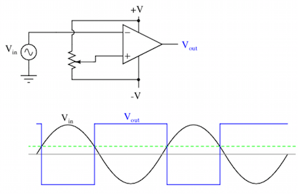
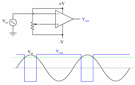
  Without feedback, the output of an op-amp is $V_{out}=A(V^+-V^-)$. As $A$ is large, $V_{out}$ is saturated, equal to either the positive or the negative voltage supply, depending on whether or not $V^+$ is greater than $V^-$. When an input of any waveform is compared with a reference voltage, the output is a square wave:

  

• A/D converter

  These two possible outputs, positive and negative, can be treated as “1” and “0” of the binary system. The figure shows an A/D converter built by three op-amps to measure voltage $V_{in}$ from 0 to 3 volts with resolution 1 V.

  

  Due to the voltage divider, the input voltages to the three op-amps are, respectively, 2.5V, 1.5V and 0.5V. The output of these op-amps are listed below for each of the input voltage levels. A digital logic circuit (a decoder) can convert the 3-bit output of the op-amps to the 2-bit binary representation.

  $$\begin{array}{c\vert\vert c\vert c\vert c\vert c}\hline \mbox... ...inary Representation} & 00 & 01 & 10 & 11 \\ \hline \end{array}$$ (57)

• Integrator and differentiator

  

  Integrator

  In time domain, as $v^-=v^+=0$ and $i_R+i_C=0$, we have (KCL)

  $$i_R+i_C=\frac{v_i}{R}+C\frac{d v_{out}}{dt}=0, \;\;\;\; \;\;\;\;v_{out}=-\frac{1}{\tau} \int v_i dt$$ (58)

  where $\tau \stackrel{\triangle}{=}RC$. In frequency domain, we have:

  $$H(j\omega)=-\frac{Z_2(j\omega)}{Z_1(j\omega)}=-\frac{1/j\omega C}{R} =-\frac{1}{j\omega RC}=-\frac{1}{j\omega \tau}$$ (59)

  Differentiator

  If we swap the resistor and the capacitor, we get in time domain:

  $$i_R+i_C=\frac{v_{out}}{R}+C\frac{d v_i}{dt}=0,\;\;\;\; \;\;\;\;v_{out}=-RC \frac{d v_i}{dt}=-\tau \frac{d v_i}{dt}$$ (60)

  In frequency domain, we have:

  $$H(j\omega)=-\frac{Z_2(j\omega)}{Z_1(j\omega)}=-\frac{R}{1/j\omega C} =-j\omega \tau$$ (61)

• PID controller

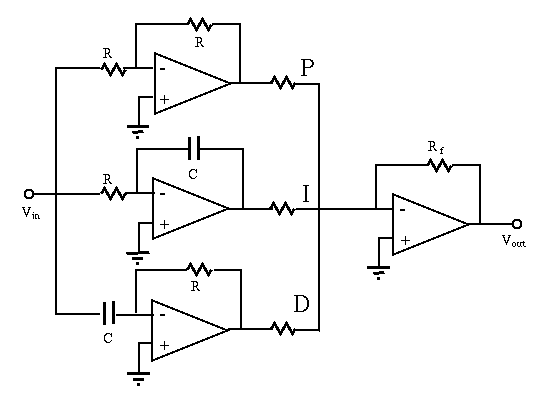
  A proportional-integral-derivative (PID) controller can be implemented as shown. The output of the circuit is a linear combination of the signal together with its integral and derivative:

  $$v_{out}(t)=c_p v_{in}(t)+c_i \int v_{in}(t) dt +c_d\frac{d\,v_{in}}{dt}$$ (62)

  

• Howland Current Source

  

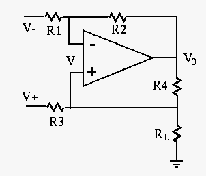
  Assuming $R_2/R_1=R_4/R_3$, we can show that the output current through the load $R_L$ is a constant determined by the input voltages $V^-$ and $V^+$, as well as the circuit parameters (see here):

  $$I_L=\frac{V^+-V^-}{R_3}=\frac{V}{R_L}$$ (63)

• Logarithmic and Exponential Amplifiers

  

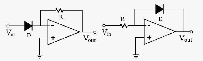
  Based on the relationship between the current through and voltage across a diode and the virtual ground assumption, we can show that the output voltage of the exponential amplifier (left) is approximately an exponential function of the input voltage, and the output voltage of the logarithmic amplifier (right) is approximately a logarithmic function of the input voltage:

  $$v_{out}\approx C \;\exp(v_{in}/a),\;\;\;\;\;\; v_{out}= D\; \ln (v_{in}/b)$$ (64)

  (Homework: Derive this relationship and determine the coefficients $C,\;D$ and $a,\,b$.)

Many op-amp circuits practically used can be found here.