Next: Higher order systems Up: Chapter 6: Active Filter Previous: Wien bridge
The transition between the pass-band and stop-band of a first order
filter with cut-off frequency
 is characterized by the
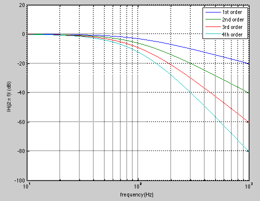
the slope of 20 dB per decade of frequency change. To achieve better
selectivity, we can cascade a set of
is characterized by the
the slope of 20 dB per decade of frequency change. To achieve better
selectivity, we can cascade a set of  such first order filters to
form an nth order filter with a slope of 20n dB per decade.
such first order filters to
form an nth order filter with a slope of 20n dB per decade.
The FRF of a first-order low-pass filter of unit gain is:
 (67)
such filters in series is (assuming they are well
buffered with no loading effect):
(67)
such filters in series is (assuming they are well
buffered with no loading effect):
 (68)
(68)
 can be
found by solving the following equation
can be
found by solving the following equation
 (69)
(69)
 (70)
(70)
Example: Design an 4th order LP filter with
 . The cut-off frequency of the
first-order LP filter can be found to be
. The cut-off frequency of the
first-order LP filter can be found to be
 (71)
(71)
 . If
. If
 ,
then
,
then
 (72)
(72)
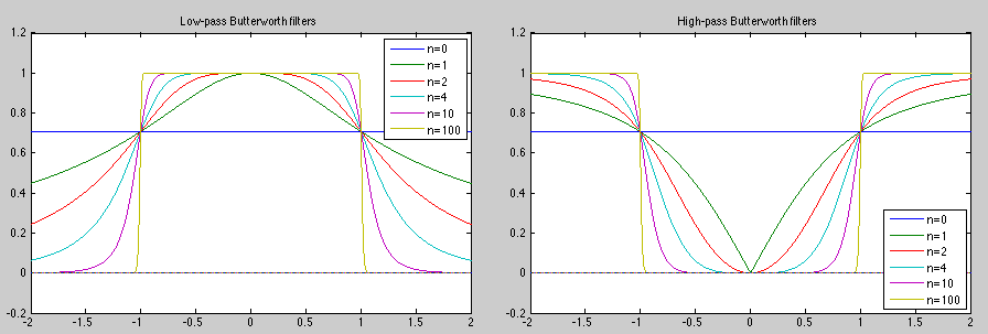
The Butterworth filters have the property that the passing
band is flat. The magnitude of the FRF of an nth order low-pass
Butterworth filter with cut-off frequency  is
is
 (73)
is the cut-off frequency at which
(73)
is the cut-off frequency at which
 .
The transition between the pass-band and stop-band is controlled by the
order . In general, higher order corresponds to more rapid transition.
Specially, when
.
The transition between the pass-band and stop-band is controlled by the
order . In general, higher order corresponds to more rapid transition.
Specially, when  ,
,  , and
, and  , we have
,
, we have
,
 is an all-pass filter.
, the Butterworth filter is the regular first-order filter:
is an all-pass filter.
, the Butterworth filter is the regular first-order filter:
 (74)
, the Butterworth filter becomes an ideal low-pass
filter:
(74)
, the Butterworth filter becomes an ideal low-pass
filter:
 (75)
(75)
The magnitude of the FRF of an nth order high-pass Butterworth filter
with cut-off frequency is
 (76)
(76)
Now we consider the implementation of a Butterworth filter. For
simplicity, in the following we assume the frequency is normalized
by the cut-off frequency , i.e.,
 ,
or
,
or  . Consider the low-pass case:
 (77)
(77)
 from its magnitude
  .
To do so, we first consider the transfer function (TF)
.
To do so, we first consider the transfer function (TF)  in the
s-domain corresponding to the FRF, which is the same as
when
in the
s-domain corresponding to the FRF, which is the same as
when  , i.e.,
 . Now the equation
above can be written as
. Now the equation
above can be written as
 (78)
and
(78)
and  , and separate them so that those on the left s-plane are
the poles of (stable and causal), while those on the right
s-plane belong to (stable and anti-causal).
, and separate them so that those on the left s-plane are
the poles of (stable and causal), while those on the right
s-plane belong to (stable and anti-causal).
The roots of the denominator can be found by solving the equation
 (79)
(79)
 solutions on the unit circle in
either of the two different forms depending on whether is even
or odd:
solutions on the unit circle in
either of the two different forms depending on whether is even
or odd:
 (80)
(80)
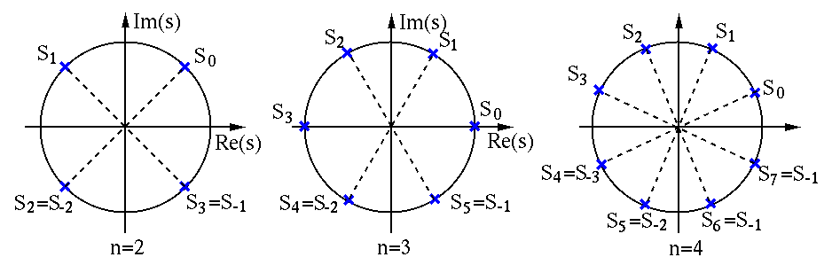
is even,
 (81)
roots form complex conjugate pairs around the unit
circle of the s-plane. Corresponding to each of the roots
(81)
roots form complex conjugate pairs around the unit
circle of the s-plane. Corresponding to each of the roots
 (
(
 ), there is another root
 that is its complex conjugate:
 (82)
to be a pole of , it needs to be on
the left s-plane, i.e.,
(82)
to be a pole of , it needs to be on
the left s-plane, i.e.,
 (83)
can be found in terms of its poles on the left s-plane:
(83)
can be found in terms of its poles on the left s-plane:
 |
 |
 |
|
|
 |
(84) |
 is the ceiling of
  , and we have
used the fact that
, and we have
used the fact that
 (85)
(85)
is odd,
 (86)
roots contain
(86)
roots contain  and
and
 , as well as
 complex conjugate pairs. Corresponding to each root
 (
(
 ), there is another root
  that is its complex
conjugate:
that is its complex
conjugate:
 (87)
(87)
 to be a pole of , it needs to be on the left s-plane, i.e.,
 (88)
can be found in terms of its poles on the left s-plane:
(88)
can be found in terms of its poles on the left s-plane:
|
|
 |
|
|
 |
(89) |
Specifically, here we find the transfer function of the nth order
Butterworth filter for  :
:
 ,
,  ,
,
 , the four roots are
 (
( ):
):
 (90)
(90)
 and
and  on the left s-plane are the roots of
:
on the left s-plane are the roots of
:
|
|
 |
|
|
 |
(91) |
 .
.
 ,
,  ,
,
 , the six roots are
 (
( )
)
 (92)
(92)
 (93)
(93)
 ,
,  , and
, and  on the left s-plane
are the roots of :
on the left s-plane
are the roots of :
|
|
 |
|
|
 |
(94) |
 .
.
 ,
,  ,
,
 , the eight roots are
 (
( ).
Evaluating
).
Evaluating
 for
for  and
and  , we get the
coefficients of the two first order terms
, we get the
coefficients of the two first order terms
 and
and
 .
.
 (95)
(95)
 ,
,  ,
,
 , the 10 roots are
 (96)
(96)
 for and , we get the
coefficients of the two first order terms
for and , we get the
coefficients of the two first order terms
 and
and
 , and we get
 (97)
(97)
 ,
,  ,
,
 , the 12 roots are
 (98)
for ,
(98)
for ,  , and
, and  ,
we get the coefficients of the three first order terms
,
we get the coefficients of the three first order terms
 ,
,
 , and
, and
 .
.
 (99)
(99)
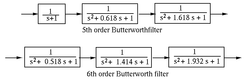
 if is even, and an additional first order system in the form of
 if is odd. The block diagrams below are for the 5th
and 6th order Butterworth filters:
if is odd. The block diagrams below are for the 5th
and 6th order Butterworth filters:
The first order filter in the cascade of the Butterworth filter can be realized by the first order op-amp low-pass circuit shown above with
 (100)
(100)
 . If we let
  , we get
 .
.
The second order systems in the cascade can be implemented as a Sallen-Key low-pass filter with
 (101)
(101)
 . If we let
  for simplicity,
we get
for simplicity,
we get
 (102)
(102)
 (103)
(103)
A High-pass Butterworth filter can be similarly implemented with the only difference that all first and second order systems in the cascade are high-pass filters
 (104)
(104)
 (105)
(105)
To convert the results obtained above for normalized cut-off frequency
 to unnormalized cut-off frequency
  , all we
need to do is to scale all capacitances
, all we
need to do is to scale all capacitances  to
to  . The
capacitor in the first order filter becomes so that
. The
capacitor in the first order filter becomes so that
 ; while the two capacitors in the second order
filter become
; while the two capacitors in the second order
filter become
 and
and
 so that
 .
.