Solving RLC Circuits by Laplace Transform

In general, the relationship of the currents and voltages in an AC circuit are described by linear constant coefficient ordinary differential equations (LCCODEs). But if only the steady state behavior of circuit is of interested, the circuit can be described by linear algebraic equations in the s-domain by Laplace transform method.

Example: A low-pass filter composed of two inductors $L$ and a capacitor $C$ is inserted between the power supply and the appliance modeled by resistor $R$ to filter out possible spikes (due to surges in the power line or lightning). 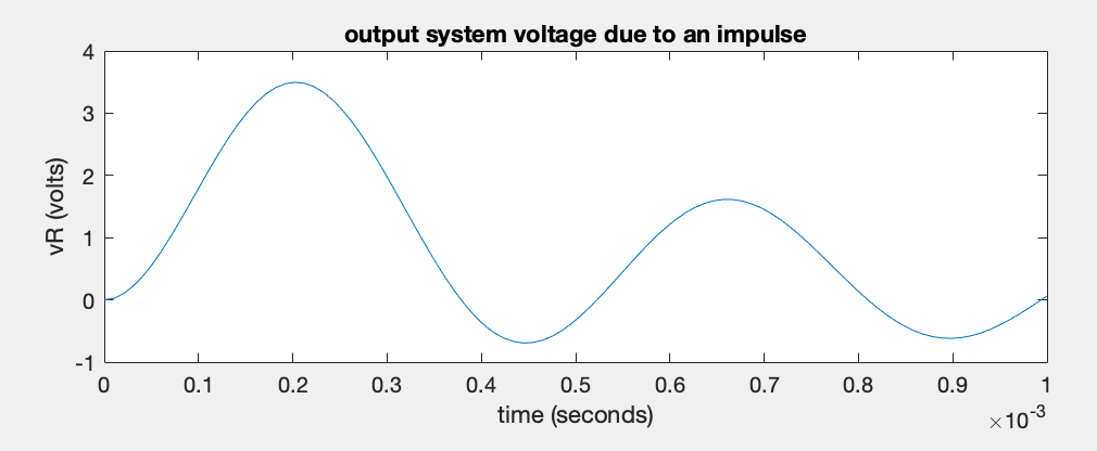Such spikes can be modeled as a square impulse of certain height, e.g., $100=10^2$ Volt and certain duration, e.g., $10 \;\mu s=10^{-5}\;sec$, which can be mathematically represented by a delta function as the input $v_s(t)=10^{-3}\delta(t)$, and we want to find out the output voltage $v_R(t)$ across the load resistor $R$ as the response to the impulse input.

Time domain: We use node-voltage method applied to the middle node $v_C$ and the output node $v_R$:

KCL to node $v_C(t)$: $i_{L1}+i_C+i_{L2}=0$, where

$$i_{L1}=\frac{1}{L_1}\int_{-\infty}^t (v_C-v_S)d\tau,\;\;\; i_{L2}=\frac{1}{L_2}\int_{-\infty}^t (v_C-v_R)d\tau,\;\;\; i_C=C\frac{dv_C}{dt}$$ (294)

$$\frac{d}{dt}(i_{L1}+i_{L2}+i_{L2}) =\frac{v_C-v_S}{L_1}+\frac{v_C-v_R}{L_2}+\frac{d}{dt}i_C=0$$ (295)

KCL to node $v_R(t)$: $i_{L2}+i_R=0$, where

$$i_{L2}=\frac{1}{L_2}\int_{-\infty}^t (v_R-v_C)d\tau,\;\;\; i_R=\frac{v_R}{R}$$ (296)

$$\frac{d}{dt}(i_{L2}+i_{L2})=\frac{v_R-v_C}{L_2}+\frac{\dot{v}_R}{R}=0$$ (297)

These differential equations can be combined to for a first order differential equation system:

$$\frac{d}{dt}\left[\begin{array}{c}v_R\\ v_C\\ i_C\end{array}\righ... ... i_C\end{array}\right] +\left[\begin{array}{c}0\\ 0\\ v_s/L_1\end{array}\right]$$ (298)

This first order ODE system can be written in generic form:

$$\dot{\bf y}={\bf Ay}+{\bf x}$$ (299)

with a general solution:

$${\bf y}=e^{{\bf A}t}{\bf y}_0+\int_0^t e^{{\bf A}(t-\tau)} {\bf x}(\tau)\;d\tau$$ (300)

Given the zero initial condition ${\bf y}(0)={\bf0}$ and an input ${\bf x}(t)=[0,\;0,\;10^{-3}\delta(t)/L_1]^T$, we can get

$$v_R=[1\;0\;0]{\bf y}=e^{{\bf A}t} \left[\begin{array}{c}0\\ 0\\ 10^{-3}/L_1\end{array}\right]$$ (301)

where

$$e^{{\bf A}t}={\bf V}e^{{\bf\Lambda}t}{\bf V}^{-1}$$ (302)

with ${\bf\Lambda}=diag(\lambda_1,\;\lambda_2,\;\lambda_3)$ and ${\bf V}=[{\bf v}_1,\;{\bf v}_2,\;{\bf v}_3]$ being the eigenvalue and eigenvector matrices of ${\bf A}$ satisfying ${\bf Av}_i=\lambda_i{\bf v}_i,\;\;(i=1,2,3)$, i.e., ${\bf A}={\bf V\Lambda V}^{-1}$.

s-domain:

$$\left\{ \begin{array}{l} \frac{V_C-V_s}{sL}+\frac{V_C}{1/sC}+... ...{sL}=0\\ \frac{V_R-V_C}{sL}+\frac{V_R}{R}=0 \end{array}\right.$$ (303)

Solving the second equation for $V_R$, we get

$$V_R=V_C\frac{R}{R+sL}$$ (304)

Substituting into the first equation, we get

$$[(R+sL)(1+LC s^2)+sL]V_C(s)=(R+sL)V_s(s)$$ (305)

Solving for $V_C$ we get

$$V_C(s)=\frac{R+sL}{(R+sL)(1+LCs^2)+sL}V_s$$ (306)

and

$$V_R(s)=V_C(s)\frac{R}{R+sL}=\frac{R}{(R+sL)(1+LCs^2)+sL}V_s$$ (307)

The voltage $v_R(t)={\cal L}^{-1}[\;V_R(s)\;]$ can be found by inverse Laplace transform.