Linear Regression

The method of regression can be used to model the relationship between an independent variable $x$ and a dependent variable $y$ by a function $y=f(x)$, based on a set of observed data pairs $\{(x_i,\,y_i)\;(i=1,\cdots,N)\}$. If there is the reason to believe that this is a linear relationship, then we can assume $\hat{y}=f(x)=w_0+w_1 x$, where the two model parameters $w_0$ (intercept) and $w_1$ (slope) are to be found for the model to fit the given data optimally, in the sense that the total squared error below is minimized:

  $$\varepsilon=\frac{1}{2}\sum_{i=1}^N r_i^2 =\frac{1}{2}\sum_{i=1}^N (y_i-\hat{y}_i)^2 =\frac{1}{2}\sum_{i=1}^N[y_i-(w_0+w_1\,x_i)]^2$$ (65)

where $r_i=y_i-\hat{y_i}=y_i-w_0+w_1 x_i$ is the residual of the ith data pair, assumed to be an i.i.d. sample of a normal distribution ${\cal N}(0,\sigma^2)$. To find the optimal coefficients $w_0$ and $w_1$ that minimize the squared error $\varepsilon$, we set its derivatives with respect to $w_0$ and $w_1$ to zero:

$$\frac{\partial \varepsilon}{\partial w_0} = -\sum_{i=1}^N(y_i-w_0-w_1\,x_i) =-\left(\sum_{i=1}^N y_i-Nw_0-w_1\sum_{i=1}^N x_i\right)$$

$$= -N( \bar{y}-w_0-w_1\bar{x} )=0$$

$$\frac{\partial \varepsilon}{\partial w_1} = -\sum_{i=1}^N(y_i-w_0-w_1\,x_i)x_i =-\left(\sum_{i=1}^N x_iy_i-w_0\sum_{i=1}^N x_i-w_1\sum_{i=1}^N x_i^2\right)$$

$$= -N\left(\frac{1}{N}\sum_{i=1}^Nx_iy_i-w_0\bar{x}-w_1\frac{1}{N}\sum_{i=1}^Nx_i^2\right)=0$$

and solve the equations to get:

  $$w_1=\frac{S_{xy}^2}{S_x^2} \;\;\;\;\;\;\;\;\;\;\;\;\;\; w_0=\bar{y}-\bar{x}\;\frac{S_{xy}^2}{S_x^2}=\bar{y}-\bar{x}\;w_1 \nonumber$$  

where

$$\bar{x} = \frac{1}{N}\sum_{i=1}^Nx_i,\;\;\;\;\;\bar{y}=\frac{1}{N}\sum_{i=1}^Ny_i$$

$$S_x^2 = \frac{1}{N}\sum_{i=1}^N(x_i-\bar{x})^2=\frac{1}{N}\sum_{i=1}^N x_i^2-\bar{x}^2$$

$$S_y^2 = \frac{1}{N}\sum_{i=1}^N(y_i-\bar{y})^2=\frac{1}{N}\sum_{i=1}^N y_i^2-\bar{y}^2$$

$$S_{xy}^2 = \frac{1}{N}\sum_{i=1}^N(x_i-\bar{x})(y_i-\bar{y}) =\frac{1}{N}\sum_{i=1}^Nx_iy_i-\bar{x}\bar{y}$$

The regression function becomes:

  $$\hat{y}=f(x)=w_0+w_1 x=\bar{y}-\bar{x}\;\frac{S_{xy}^2}{S_x^2} +\frac{S_{xy}^2}{S_x^2}x =\bar{y}+\frac{S_{xy}^2}{S_x^2}(x-\bar{x}) \nonumber$$  

We see that the slope of the linear regression function can also be written as

  $$w_1=\frac{S_{xy}^2}{S_x^2}=\frac{y-\bar{y}}{x-\bar{x}} \nonumber$$  

The univariate linear regression model considered above can be generalized to multivariate linear regression, by which the relationship between a dependent variable $y$ and $D$ independent variables $\{ x_1,\cdots,x_D\}$ is modeled by a linear function

  $$\hat{y}=f( x_1,\cdots,x_D)=w_0+\sum_{d=1}^D x_d w_d =\sum_{d=0}^D x_d w_d$$ (66)

where $x_0=1$. We desire to find the $D+1$ model parameters $\{w_0,\,w_1,\cdots,w_D\}$ so that the model fits optimally a set of observed sample points $\{ (x_{n1},\cdots,x_{nD},y_n)\; (n=1,\cdots,N)\}$. Substituting the observed data into the model we get $N$ equations

  $$\hat{y}_n=\sum_{d=0}^D x_{nd} w_d,\;\;\;\;\;\;\;(n=1,\cdots,N)$$ (67)

which can be written in matrix form:

$$\hat{\bf y} = \left[\begin{array}{c}\hat{y}_1\\ \vdots\\ \hat{y}_N\end{array}... ...{\bf x}_D] \left[\begin{array}{c} w_0\\ w_1\\ \vdots\\ w_D\end{array}\right]$$

$$= {\bf Xw}=\sum_{d=0}^D w_d{\bf x}_d$$

where we have defined

  $${\bf w}=\left[\begin{array}{c}w_0\\ w_1\\ \vdots\\ w_D\end{array}... ...\;\;\;\; {\bf X}=[{\bf x}_0={\bf 1},{\bf x}_1,\cdots,{\bf x}_D]_{N\times(D+1)}$$ (68)

Ideally, we want to find ${\bf w}$ so that ${\bf y}=\hat{\bf y}={\bf Xw}=\sum_{d=0}^D w_d{\bf x}_d$, i.e., the observed ${\bf y}$ can be expressed as a linear combination of $D+1$ vectors $\{{\bf x}_0={\bf 1},{\bf x}_1,\cdots,{\bf x}_D\}$. However, as this is an over determined equation system with $N$ equations but only $D+1 < N$ unknowns $\{w_0,w_1,\cdots,w_D\}$, there does not exist an exact solution. We therefore can only find the least square (LS) approximation that minimizes the residual ${\bf r}={\bf y}-\hat{\bf y}$, the squared error:

$$\varepsilon({\bf w}) = \frac{1}{2} =\frac{1}{2}\vert\vert{\bf r}\vert\vert^2 =\frac{1}{2}{\bf r}^T{\bf r} =\frac{1}{2}({\bf y}-{\bf Xw})^T({\bf y}-{\bf Xw})$$

$$= \frac{1}{2}\left({\bf y}^T{\bf y}-2({\bf Xw})^T{\bf y} +{\bf w}^T{\bf X}^T{\bf Xw}\right)$$ (69)

To do so, we find its gradient (derivatives) with respect to ${\bf w}=[w_0,w_1,\cdots,w_D]^T$ to zero:

  $${\bf g}_\varepsilon({\bf w})=\frac{d\varepsilon({\bf w})}{d{\bf w... ...}+{\bf X}^T{\bf Xw} =-{\bf X}^T({\bf y}-\hat{\bf y})=-{\bf X}^T{\bf r}={\bf0}$$ (70)

and solve the resulting equation to get:

  $${\bf w}=({\bf X}^T{\bf X})^{-1}{\bf X}^T{\bf y}={\bf X}^-{\bf y}$$ (71)

where ${\bf X}^-=({\bf X}^T{\bf X})^{-1}{\bf X}^T$ is the $(D+1)\times N$ pseudo-inverse of ${\bf X}$.

We further consider some properties of the solution. First, we note that

  $${\bf X}^T{\bf r}=\left[\begin{array}{c}{\bf x}_0^T\\ {\bf x}_1^T\\ \vdots\\ {\bf x}_D^T\end{array}\right]{\bf r}={\bf0}$$ (72)

of which the first component is

  $${\bf x}_0^T{\bf r}=[1,\cdots,1]{\bf r}=\sum_{n=1}^N r_n=0$$ (73)

i.e., the sum of all $N$ residuals is zero. Now the regression model can be written as $\hat{\bf y}={\bf Xw}={\bf XX}^-{\bf y}$, and we have

  $$\hat{\bf y}^T\hat{\bf y} =\left({\bf Xw}\right)^T\left({\bf X}{\b... ...T{\bf X})^{-1}{\bf X}^T{\bf y} ={\bf w}^T{\bf X}^T{\bf y}=\hat{\bf y}^T{\bf y}$$ (74)

and

$${\bf r}^T{\bf r} = ({\bf y}-\hat{\bf y})^T({\bf y}-\hat{\bf y}) ={\bf y}^T{\bf y}-2{\bf y}^T\hat{\bf y}+\hat{\bf y}^T\hat{\bf y}$$

$$= {\bf y}^T{\bf y}-2{\bf y}^T\hat{\bf y}+\hat{\bf y}^T{\bf y} ={\bf y}^T{\bf y}-{\bf y}^T\hat{\bf y} ={\bf y}^T({\bf y}-\hat{\bf y})={\bf y}^T{\bf r}$$

i.e.,

  $${\bf r}^T{\bf r}={\bf r}^T({\bf y}-\hat{\bf y}) ={\bf r}^T{\bf y}-{\bf r}^T\hat{\bf y}={\bf y}^T{\bf r}$$ (75)

we therefore get

  $${\bf r}^T\hat{\bf y}=({\bf y}-\hat{\bf y})^T\hat{\bf y}=0 \;\;\;\;\;\;\mbox{i.e.}\;\;\;\;\;\;\; \hat{\bf y}^T\hat{\bf y}={\bf y}^T\hat{\bf y}$$ (76)

We can also show that all three vectors ${\bf y}-\hat{\bf y}$, ${\bf y}-\bar{\bf y}$ and $\hat{\bf y}-\bar{\bf y}$ are perpendicular to vector ${\bf 1}=[1,\cdots,1]^T$:

$$({\bf y}-\bar{\bf y})^T{\bf 1} = \sum_{n=1}^N(y_n-\bar{y}) =N(\bar{y}-\bar{y})=0$$

$$({\bf y}-\hat{\bf y})^T{\bf 1} = \sum_{n=1}^N(y_n-\hat{y}_n) =\sum_{n=1}^N r_n=0$$

$$(\hat{\bf y}-\bar{\bf y})^T{\bf 1} = (\hat{\bf y}-{\bf y}+{\bf y}-\bar{\bf y})^T{\bf 1} =(\hat{\bf y}-{\bf y})^T{\bf 1}+({\bf y}-\bar{\bf y})^T{\bf 1} =0$$ (77)

The fact that the residual ${\bf r}={\bf y}-\hat{\bf y}$ is perpendicular to ${\bf y}$ indicates that among all linear combinations of the $D+1$ vectors $\{{\bf x}_0={\bf 1},{\bf x_1} \cdots,{\bf x}_D\}$ (all points on the hypersurface spanned by these vectors), $\hat{y}={\bf X}^-{\bf y}$ is indeed the optimal one with the minimum residual ${\bf r}$.

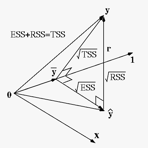
How well the regression model fits the observed data can be quantitatively measured based on the following sums of squares:

• The total sum of squares (SST): The total variation in the data
    $$SST=\vert\vert{\bf y}-\bar{\bf y}\vert\vert^2=\sum_{i=1}^n(y_i-\bar{y})^2$$ (78)

• The explained sum of squares (SSE): variation of data explained by the regression model:
    $$SSE=\vert\vert\hat{\bf y}-\bar{\bf y}\vert\vert^2=\sum_{i=1}^n(\hat{y}_i-\bar{y})^2$$ (79)
• Residual sum of squares (SSR): variation of data not explained by the data, due to the noise, or discrepancy between the data and the model:
    $$SSR=\vert\vert{\bf y}-\hat{\bf y}\vert\vert^2=\vert\vert{\bf r}\vert\vert^2$$ (80)

We can show that the total sum of squares is the sum of the explained sum of squares and the residual sum of squares:

$$SST = \vert\vert{\bf y}-\bar{\bf y}\vert\vert^2 =\vert\vert{\bf y}-\bar... ...t\vert^2 =\vert\vert(\hat{\bf y}-\bar{\bf y})+({\bf y}-\hat{\bf y})\vert\vert^2$$

$$= \vert\vert\hat{\bf y}-\bar{\bf y}\vert\vert^2 +2({\bf y}-\hat{\bf y})^T(\hat{\bf y}-\bar{\bf y}) +\vert\vert{\bf y}-\hat{\bf y}\vert\vert^2$$

$$= \vert\vert\hat{\bf y}-\bar{\bf y}\vert\vert^2+2{\bf r}^T(\hat{\bf y}-\bar{\bf y})+\vert\vert{\bf r}\vert\vert^2$$

$$= SSE+2{\bf r}^T\hat{\bf y}-2{\bf r}^T\bar{\bf y}+SSR =SSE+SSR$$

The last equality is due to the fact that the two middle terms are both zeros:

  $${\bf r}^T\hat{\bf y}=0,\;\;\;\;\;\;\;\; {\bf r}^T\bar{\bf y}=\sum_{n=1}^Nr_n\bar{y} =\bar{y}\sum_{n=1}^Nr_n=0$$ (81)

We now define the coefficient of determination denoted by $R^2$ (R-squared) as a measure for the goodness of the model as the percentage of variance explained by the model:

  $$R^2=\frac{SSE}{SST}=1-\frac{SSR}{SST}$$ (82)

If SSR is small, i.e., the model residual is small, then SSE is large, i.e., most of the variation in the data can be explained by the model, then $R^2$ is large, indicating a good fit of the model to the data.

In particular, when $D=1$, we find the parameters of the linear regression model $\hat{y}=w_0+w_1 x$, the slope $w_1=S^2_{xy}/S_x^2$ and the intercept $w_0=\bar{y}-\bar{x} w_1$. We may ask two different questions regarding the data and the model:

• How closely are the two variables $x$ and $y$ related to each other? This question can be addressed by the correlation coefficient defined as:
    $$\rho=\frac{\sum_{i=1}^N(x_i-\bar{x})(y_i-\bar{y})} {\sqrt{\sum_{... ...\bar{y})^2}} =\frac{S_{xy}^2}{\sqrt{S_x^2\;S_y^2}}=\frac{S_{xy}^2}{S_x\;S_y}$$ (83)
  A few simple examples of different correlation coefficients can be found here.

• How well does the regression model fits the observed data? This question can be addressed by the goodness measure $R^2$ discussed above.

In fact, $\rho$ for correlation and $R^2$ for regression are closely related. Specifically, consider

$$SSR = \vert\vert{\bf y}-\hat{\bf y}\vert\vert^2=\sum_{n=1}^N(y_n-w_0-w_1x_n)^2 =\sum_{n=1}^N(y_n-(\bar{y}-\bar{x} w_1)-w_1x_n)^2$$

$$= \sum_{n=1}^N[(y_n-\bar{y})-w_1(x_n-\bar{x})]^2 =\sum_{n=1}^N[(y_n-\bar{y})^2-2w_1(y_n-\bar{y})(x_n-\bar{x}) +w_1^2(x_n-\bar{x})^2]$$

$$= S_y^2-2w_1S^2_{xy}+w_1^2S_x^2 =S_y^2-2\frac{S_{xy}^2}{S^2_x}S^2_{... ..._{xy}}{S^2_x} =S_y^2\left(1-\frac{S^4_{xy}}{S_x^2S_y^2}\right) =S_y^2(1-\rho^2)$$ (84)

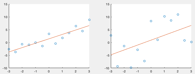
We see that if $\rho$ is large, indicating the two variables $x$ and $y$ are highly correlated, then SSR is small, i.e., the error of the model is small, therefore $R^2$ is large, indicating the model is a good fit of the data.

Although correlation and regression are closely related to each other, they are different in several aspects:

• Only if two variables $x$ and $y$ are correlated will regression analysis be meaningful.
• In regression $y$ is a dependent variable, possibly random, a function of ${\bf x}$, a deterministic independent variable. But they are treated equally (both possibly random) in correlation.
• Regression can provide a model, a specific mathematical function $y=f(x)$, by which the given samples can be interpolated and extrapolated; but correlation cannot.

Examples:

  $$\begin{tabular}{c\vert\vert c\vert c\vert c\vert c\vert c\vert c\... ...-7.29 & 8.31 & 0.98 & 10.18 & 8.58 &10.86 & 0.77 & 0.20\\ \hline \end{tabular}$$ (85)

  $$\begin{tabular}{c\vert\vert c\vert c\vert c\vert c\vert c\vert c\... ...0.91 & 1.92 & 166.98 & 443.92 & 610.89 & 0.273 & 0.523 \\ \hline \end{tabular}$$ (86)