Next: Two-Sample t-Test Up: StatisticTests Previous: Common Probability Density functions
Given an observed data set
 of
of  i.i.d
samples of a normal distribution
i.i.d
samples of a normal distribution
 of
unknown
of
unknown  and
and  , we can carry out the test of a
null hypothesis
, we can carry out the test of a
null hypothesis  claiming that the sample mean
  is the same as an expected value such as a hypothesized mean
 . As the result of the test, is either accepted
or rejected in favor of one of the alternative hypotheses
. As the result of the test, is either accepted
or rejected in favor of one of the alternative hypotheses
 :
:
:  ,
,
 :
:
 (two-tailed)
 (one-tailed-greater)
 (two-tailed-smaller)
The one-sample t-test can be used to compare the mean of a population with an expected value, to see if there exists a significant difference. Examples include, the drinking water contaminants compared with standards/regulations, test scores of a school compared to the average of all schools in the district.
To test the null hypothesis , we first find the sample mean
 (22)
is known:
(22)
is known:
 (23)
(23)
 is the standard error.
If is unknown (typically the case), we have to estimate
it by the sample variance:
 (24)
(24)
 degrees of freedom:
 (25)
(25)
 is the estimated standard error.
Evaluating  based on the calculated and
, we get the specific value
based on the calculated and
, we get the specific value  of the
test statistic. Qualitatively, a larger value of
of the
test statistic. Qualitatively, a larger value of  indicates
and are more different, and for
indicates
and are more different, and for
 is more likely to be rejected, in favor of an
alternative hypothesis , such as
is more likely to be rejected, in favor of an
alternative hypothesis , such as
 .
.
We also find the critical values
 satisfying
 and
and
 satisfying
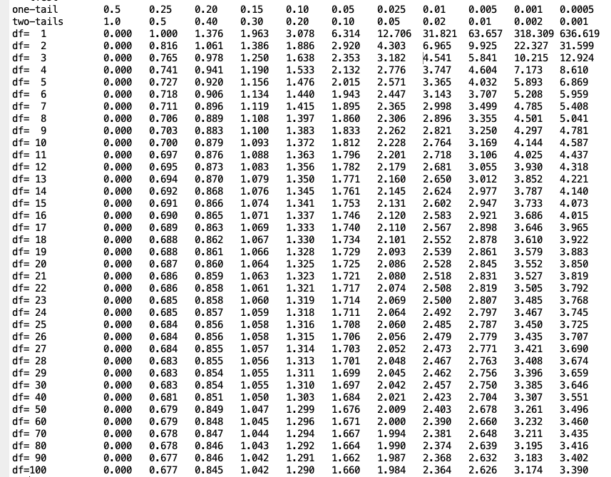
 , from the two-tailed
t-Table
of , or the Matlab inverse cumulative density
function
, from the two-tailed
t-Table
of , or the Matlab inverse cumulative density
function icdf. For example, if  and
and
 , i.e.,
  , we find
 and
and
 .
.
The probability for to fall inside the interval
![$[t_{\alpha/2},\;t_{1-\alpha/2}]$](img98.svg) is
is  :
:
 (26)
to fall inside the
critical region outside the interval above is
(26)
to fall inside the
critical region outside the interval above is
 (27)
for , depending on whether falls inside the
critical region:
(27)
for , depending on whether falls inside the
critical region:
 , is in the critical
region, indicating is significantly smaller than
, is rejected;
, is in the critical
region, indicating is significantly smaller than
, is rejected;
 , is in the critical
region, indicating is significantly greater than
, is rejected;
, is in the critical
region, indicating is significantly greater than
, is rejected;
 , is not in
the critical region, is not rejected.
, is not in
the critical region, is not rejected.
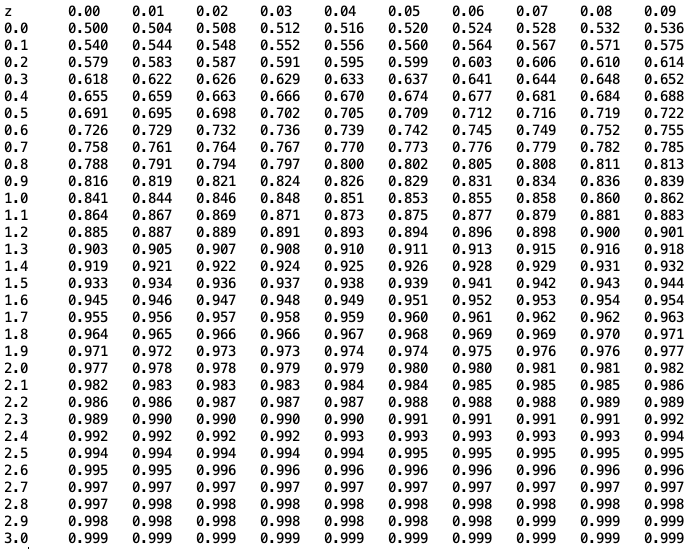
Alternatively and equivalently, we can find the p-value based
on the test statistic value , from the t-Table or the Matlab
cumulative density function cdf:
 (28)
(28)
 , or equivalently,
 , then is
inside the critical region, indicating the fact that observing this
specific is a low probability event according to the null
hypothesis , but as it did happen, then the null hypothesis
has to be rejected. On the other hand, if
, then is
inside the critical region, indicating the fact that observing this
specific is a low probability event according to the null
hypothesis , but as it did happen, then the null hypothesis
has to be rejected. On the other hand, if  , the evidence
against is not significant enough, i.e., rejecting has
chance of being wrong (but still
, the evidence
against is not significant enough, i.e., rejecting has
chance of being wrong (but still  chance of being
right), we fail to reject . However, this result is not
necessarily a significant evidence for .
chance of being
right), we fail to reject . However, this result is not
necessarily a significant evidence for .
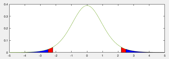
In the figure below, the one and two-tailed t-distributions of 10 d.f.
are shown. In all cases, the red area is determined by
the critical value  in one-tailed case (top) or
  in two-tailed case (bottom), the blank area underneath the pdf is
 , while the blue area is the p-value, determined by
the value of the test statistic. In both cases,the null hypothesis
is . If , is rejected, as data support the
alternative hypothesis , which is
, while the blue area is the p-value, determined by
the value of the test statistic. In both cases,the null hypothesis
is . If , is rejected, as data support the
alternative hypothesis , which is  in one-tailed case
(top-left), or
in two-tailed case (bottom-left). If
, is accepted (right).
in one-tailed case
(top-left), or
in two-tailed case (bottom-left). If
, is accepted (right).

In general, if is very different from (strong
signal), and the variance or the sample variance  is
small and sample size is large (small noise), then the absolute
value
is
small and sample size is large (small noise), then the absolute
value
 of is large, and p-value is small,
the null hypothesis is likely to be rejected.
of is large, and p-value is small,
the null hypothesis is likely to be rejected.
If is known, or if the sample size is large enough
(e.g.,  ), then the test statistic
 with t-distribution can be replaced by
 with
standard normal distribution, and the t-test above can be replaced
by a z-test.
with
standard normal distribution, and the t-test above can be replaced
by a z-test.
Example: According to the drinking water standard the maximal
allowed lead content is
 . Given samples
taken from the tap water shown below, determine whether the lead
content is significantly higher than the standard based on
.
. Given samples
taken from the tap water shown below, determine whether the lead
content is significantly higher than the standard based on
.
 (29)
(29)
The null hypothesis is
 , i.e., there is no
difference between the mean lead content level of the tap water
and the standard. The sample mean and sample standard deviation can
be found from the data samples as
, i.e., there is no
difference between the mean lead content level of the tap water
and the standard. The sample mean and sample standard deviation can
be found from the data samples as
 and
and  ,
respectively, and the test statistic value
,
respectively, and the test statistic value  is outside
the interval defined by the critical value
is outside
the interval defined by the critical value
 , i.e., is in the critical
region (red areas). Alternatively, we can find the p-value
, i.e., is in the critical
region (red areas). Alternatively, we can find the p-value
 (the blue areas), which is smaller than
(the red areas). Based on either of the two equivalent results,
we conclude that the lead content is significantly higher than
the standard.
(the blue areas), which is smaller than
(the red areas). Based on either of the two equivalent results,
we conclude that the lead content is significantly higher than
the standard.
We can also find the confidence interval of the mean
based on and  in terms of its upper and lower
limits satisfying:
in terms of its upper and lower
limits satisfying:
 (30)
(30)
 , i.e., the sample mean
is the same as the mean of the distribution, and the test statistic
is
, i.e., the sample mean
is the same as the mean of the distribution, and the test statistic
is
 .
.
If the sample size is large enough, e.g.,  , the sample
variance
, the sample
variance  can be assumed to be approximately the same as the
true variance , and the test statistic
can be assumed to be approximately the same as the
true variance , and the test statistic
 can be approximated by
 . In this case,
we can use the Z-test. Based on the z-Table
we can find the critical values
. In this case,
we can use the Z-test. Based on the z-Table
we can find the critical values  and
and
 satisfying the following:
 (31)
(31)
 |
|||
 |
 |
,
 , we can find
 .
.

We can further find the lower and upper limits of the confidence
interval for , based on the fact that the probabilities of
the following equivalent events are the same:
 |
|||
|
 |
 (32)
corresponding to the given .
(32)
corresponding to the given .
However, if the sample size is not large enough, the pdf of
the test statistic is a t-distribution with , and we
find the critical values and
 satisfying the following
 (33)
(33)
 |
|||
|
 |

For example, assuming , , and ,
we can find from the t-Table
 and
and
 , which is greater than
 based on normal distribution, due to the longer tails of the
t-distribution. When the sample size becomes larger,
based on normal distribution, due to the longer tails of the
t-distribution. When the sample size becomes larger,
 approaches the standard normal
distribution
approaches the standard normal
distribution  , and approaches .
For example, when
, and approaches .
For example, when  ,
,
 is very close to
 .
.
We can further find the lower and upper limits of the confidence
interval for , due to the fact that the probabilities of the
following equivalent events are the same:
 (34)
as:
(34)
as:
 (35)
(35)
 .
.
Example: Based on the same data set in the previous example,
we can find the critical value as
and
 , and the lower and upper limits
of the confidence interval of the mean can be found as
, and the lower and upper limits
of the confidence interval of the mean can be found as
 , i.e.,
 (36)
(36)
The Matlab function ttest can be used to carry out all
t-test discussed above.