Correlation based motion detection

Next: Gradient based motion detection Up: The Models Previous: Delay and multiply model

Correlation based motion detection

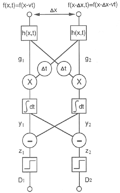
This is a more elaborate model based on the same idea as above. As shown in the figure, the two sensors (receptors) are placed with a distance $\triangle x$ apart in 1D space. A spatial pattern moving at velocity v>0 is represented by f(x,t)=f(x-vt) (v>0 for rightward motion and v<0 for the opposite direction). The responses of the light sensors to the input signals are, respectively,

$\begin{displaymath}\left\{ \begin{array}{l} g_1(x,t)=h(x,t)*f(x,t) \\ g_2(x,t)=h(x,t)*f(x-\triangle x,t) \end{array} \right. \end{displaymath}$

where h(x,t) is the impulse response of the sensors (assumed to be linear and space-time invariant) and their outputs can be found as the convolutions (represented by *) of the impulse response and the inputs. The two signals g₁ and g₂, one of which delayed by $\triangle t$ , are next multiplied and integrated with respect to time (correlation) to generate the velocity sensitive outputs:

$\begin{displaymath}\left\{ \begin{array}{l} y_1=\int g_1(t) g_2(t-\triangle t)\... ... y_2=\int g_1(t-\triangle t) g_2(t)\; dt \end{array} \right. \end{displaymath}$

The differences between y₁ and y₂ are obtained as the direction selective outputs z₁=y₁-y₂, z₂=y₂-y₁ (note that the order of integration and subtraction can be reversed), which then go through a threshold to get binary outputs D₁ and D₂ indicating whether a motion with a certain velocity is detected or not.

Let us first assume a moving pattern is a point light source $f(x,t)=\delta(x-vt)$ . Then we have

$\begin{displaymath}\left\{ \begin{array}{l} g_1=h*\delta(x-vt)=h(x-vt) \\ g_2... ...lta(x-\triangle x-vt)=h(x-\triangle x-vt) \end{array} \right. \end{displaymath}$

The correlations become

$\begin{displaymath}\left\{ \begin{array}{l} y_1=\int g_1(t) g_2(t-\triangle t)\... ...+v\triangle t) h(x-\triangle x-vt)\; dt \end{array} \right. \end{displaymath}$

Obviously, y₁ and y₂ are both functions of v, the velocity of motion. When $v=\triangle x/\triangle t$ , the two functions in the correlation for y₁ coincide and $y_1=\int \left\vert h \right\vert^2 dt$ reaches maximum, and thus indicating a motion toward right at velocity v. If v moves away from this particular value $\triangle x/\triangle t$ (becoming either larger or smaller than this value), y₁ will become smaller as the two functions in the correlation will move farther apart from each other and their overlap will become smaller, until eventually y₁ approaches zero when the two functions are so far apart that they have almost no overlap. It can be seen that y₁(v) now becomes the velocity tuning curve of this velocity sensitive unit, which can be approximated by a Gaussian function. The width of the tuning curve is related to both $\triangle x$ and $\triangle t$ . The same is true for the other output y₂, except that it detects the velocity in the opposite direction as it reaches maximum when $v=-\triangle x/\triangle t$ . After subtraction and thresholding, D₁ and D₂ are obtained to indicate whether a motion of certain velocity is present. The above analysis can be generalized from $\delta(x-vt)$ to any spatial moving pattern f(x-vt).

../figures/correlation_model.gif

Next, we consider a sinusoidal signal $cos(\omega (x-vt))$ , where $\omega$ is its spatial frequency. (Strictly speaking, a constant needs to be added to make the pattern non-negative) The outputs of the linear system (steady state) are known to be also sinusoidal:

$\begin{displaymath}\left\{ \begin{array}{l} g_1(t)= \left\vert H \right\vert co... ...os(\omega (x-\triangle x-vt) + \angle H) \end{array} \right. \end{displaymath}$

where $\left\vert H \right\vert$ and $\angle H$ are, respectively, the magnitude and phase angle of the transfer function H of the light sensor h. Trigonometric identities can be used to obtain the final results after integration and subtraction:

$\begin{displaymath}z_1,z_2= \pm \left\vert H \right\vert^2 sin(\omega \triangle x) sin(\omega v\triangle t)\end{displaymath}$

These outputs are sinusoidal functions of the motion velocity v (with other parameters $\triangle x$ , $\triangle t$ and $\omega$ fixed), and they reach maximum $\left\vert H \right \vert^2 sin^2(\omega \triangle x)$ when $v=\pm \triangle x/\triangle t$ . After going through the threshold the outputs D₁ and D₂ will be either positive to indicate a preferred motion direction, or zero for the opposite direction (null direction). By Fourier theory, this result can be generalized for any periodical spatial functions.

Moreover, the above model for 1D motion can be easily generalized to detect 2D motions. More detailed discussion of this model can be found in [20].

Next: Gradient based motion detection Up: The Models Previous: Delay and multiply model

Ruye Wang
2000-04-25