Definition of DCT

The discrete Fourier transform (DFT) transforms a complex signal into its complex spectrum. However, if the signal is real as in most of the applications, half of the data is redundant. In time domain, the imaginary part of the signal is all zero; in frequency domain, the real part of the spectrum is even symmetric and imaginary part odd. In comparison, Discrete cosine transform (DCT) transforms is a real transform that transforms a sequence of real data points into its real spectrum and therefore avoids the problem of redundancy. Also, as DCT is derived from DFT, all the desirable properties of DFT (such as the fast algorithm) are preserved.

To derive the DCT of an N-point real signal sequence $\{x[0],\cdots,x[N-1]\}$, we first construct a new sequence of $2N$ points:

$$x'[m]\stackrel{\triangle}{=}\left\{ \begin{array}{ll} x[m] ... ...\leq N-1) x[-m-1] & (-N \leq m \leq -1) \end{array} \right.$$

This 2N-point sequence $x'[m]$ is assumed to repeat its self outside the range $-N \leq n \leq N-1$, i.e., it is periodic with period $2N$, and it is even symmetric with respect to the point at $m=-1/2$:

$$x'[m]=x'[-m-1]=x'[2N-m-1]$$

If we shift the points $x'[m]$ to the right by 1/2, or, equivalently, shift $m$ to the left by 1/2 by defining another index $m'=m+1/2$, then $x'[m]=x'[m'-1/2]$ is even symmetric with respect to the origin at $m'=0$. In the following we simply represent this new function by $x[m]$.

The DFT of this 2N-point even symmetric sequence can be found as:

$$X[n] = \frac{1}{\sqrt{2N}} \sum_{m'=-N+1/2}^{N-1/2} x\left[m'-\frac{1}{2}\right]e^{-j2\pi m'n/2N}$$

$$= \frac{1}{\sqrt{2N}} \sum_{m'=-N+1/2}^{N-1/2}x\left[m'-\frac{1}{2}... ...+1/2}^{N-1/2}x\left[m'-\frac{1}{2}\right]\;\sin\left(\frac{2\pi m'n}{2N}\right)$$

$$= \frac{1}{\sqrt{2N}} \sum_{m'=-N+1/2}^{N-1/2}x\left[m'-\frac{1}{2}... ...2}\right]\;\cos\left(\frac{2\pi m'n}{2N}\right) \;\;\;\;\;\;\;(n=0,\cdots,2N-1)$$

Here we have used the fact that $x[m'-1/2]$ is even, $\cos(2\pi m'n/2N)$ and $\sin(2\pi m'n/2N)$ are respectively even and odd, all with respect to $m'=0$ or $m=-1/2$. Consequently the first summation of all even terms is twice that with half of the range $m'=1/2,\cdots,N-1/2$, while the second summation of all odd terms is zero. Replacing $m'$ by $m+1/2$, we get the discrete cosine transform (DCT):

$$X[n] = \sqrt{\frac{2}{N}} \sum_{m'=1/2}^{N-1/2}x\left[m'-\frac{1}{2}\rig... ...\sqrt{\frac{2}{N}} \sum_{m=0}^{N-1}x[m]\;\cos\left(\frac{(2m+1)n\pi}{2N}\right)$$

$$= \sum_{m=0}^{N-1} c[n,m]x[m],\;\;\;\;\;\;\;\;\;(n=0,\cdots,N-1)$$

where the coefficient $c[n,m]$ defined as

$$c[n,m]\stackrel{\triangle}{=}\sqrt{\frac{2}{N}}\cos\left(\frac{ (2m+1)n\pi}{2N}\right), \;\;\;\;\;\;\;(m,n=0,1,\cdots,N-1)$$

which can be considered as the component on the mth row and nth column of an $N\times N$ matrix ${\bf C}$, called the DCT matrix.

As $X[n]=X[-n]$ is even and of period $2N$, we further have

$$X[N+n]=X[N+n-2N]=X[n-N]=X[N-n]$$

i.e., the second $N$ coefficients $X[n]$ for $n=N,\cdots,2N-1$ are redundant and can be dropped. Now the the range for index $n$ is reduced to $n=0,\cdots,N-1$. We can show that all row vectors of ${\bf C}$ are orthogonal and normalized, except the first one ($n=0$):

$$\sqrt{\sum_{m=0}^{N-1}c^2[n,m]}= \sqrt{\frac{2}{N} \sum_{m=0}... ...qrt{2} &\;\;n=0 1 &\;\;n=1,2,\cdots,N-1 \end{array} \right.$$

To make DCT a orthonormal transform, we define a coefficient

$$a[n]=\left\{ \begin{array}{ll} \sqrt{1/N} & \;\;n=0 \sqrt{2/N} &\;\; n=1,2,\cdots,N-1 \end{array} \right.$$

so that the DCT now becomes

$$X[n] = a[n] \sum_{m=0}^{N-1}x[m]\;\cos\left(\frac{ (2m+1)n\pi... ...) =\sum_{m=0}^{N-1}x[m]\;c[n,m]\;\;\;\;\;\;\;(n=0,\cdots,N-1)$$

where $c[n,m]$ is modified with $a[n]$, which is also the component in the nth row and mth column of the N by N cosine transform matrix:

$$\left[ \begin{array}{ccc} \cdots & \cdots & \cdots \\ \vdot... ...T \vdots {\bf c}_{N-1}^T \end{array} \right] ={\bf C}^T$$

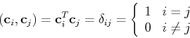
Here ${\bf c}_i^T=[c[i,0],\cdots,c[i,N-1]$ is the ith row of the DCT transform matrix ${\bf C}$. As these row vectors are orthogonal:

$$({\bf c}_i,{\bf c}_j)={\bf c}_i^T {\bf c}_j =\delta_{ij} =\left\{ \begin{array}{ll}1 & i=j 0 & i\ne j \end{array} \right.$$

the DCT matrix ${\bf C}$ is orthogonal:

$${\bf C}^{-1}={\bf C}^T,\;\;\;\;\mbox{i.e.} \;\;\;\;{\bf C}^T {\bf C}= {\bf I}$$

and it is real ${\bf C}={\bf C}^*$. Now the DCT can be expressed in matrix form as:

$${\bf X}={\bf C}^T {\bf x}$$

Left multiplying both sides by ${\bf C}$ we get

$${\bf C}{\bf X}={\bf C}{\bf C}^T{\bf x}={\bf C}{\bf C}^{-1}{\bf x}={\bf x}$$

this is the inverse DCT:

$${\bf x}={\bf C}{\bf X}$$

or in component form:

$$x[m] = \sum_{n=0}^{N-1} X[n]\;c[m,n]= \sum_{n=0}^{N-1} a[n] X... ...t) =\sum_{n=0}^{N-1}X[n]\;c[n,m]\;\;\;\;\;\;\;(m=0,\cdots,N-1)$$

Example: When $N=2$, we have $c[n,m]=a[n]\cos((2m+1)n\pi/4)$ for $m,n=0,1$, and

$${\bf C}=\frac{1}{\sqrt{2}}\left[\begin{array}{cr} 1 & 1 1 & -1\end{array}\right]$$

An $N=4$-point DCT matrix can be generated by $c[n,m]=a[n] cos( (2m+1)n\pi/8)$ to be

$${\bf C}^T=\left[ \begin{array}{c} {\bf c}_0^T \vdots {\... ....50 & 0.50 \\ 0.27 & -0.65 & 0.65 & -0.27 \end{array} \right]$$

Assume the signal is ${\bf x}=[0\; 1\; 2\; 3]^T$, then its DCT transform is:

$${\bf X}={\bf C}^T {\bf x}=\left[ \begin{array}{rrrr} 0.50 & ... ...egin{array}{r} 3.00 -2.23 0.00 -0.16 \end{array} \right]$$

The inverse transform is:

$${\bf x}={\bf C} {\bf X}=\left[ \begin{array}{rrrr} 0.50 & 0.... ...ht] =\left[ \begin{array}{r} 0 1 2 3 \end{array} \right]$$

This result is very similar to the example shown in the previous section for WHT transform. In fact, these two transforms are very comparable, as seen from the figure below:

Compared with DFT, DCT has two main advantages:

• It is a real transform with better computational efficiency than DFT which by definition is a complex transform.
• It does not introduce discontinuity while imposing periodicity in the time signal. In DFT, as the time signal is truncated and assumed periodic, discontinuity is introduced in time domain and some corresponding artifacts is introduced in frequency domain. But as even symmetry is assumed while truncating the time signal, no discontinuity and related artifacts are introduced in DCT.