Next: Appendix
Up: algebra
Previous: Vector and matrix differentiation
In general an over-determined linear equation system of  unknowns but
 equations has no solution if
  . But it is still possible to find the
optimal approximation in the least squares sense, so that the squared error is
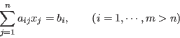
minimized. Specifically, consider an over determined linear equation system
. But it is still possible to find the
optimal approximation in the least squares sense, so that the squared error is
minimized. Specifically, consider an over determined linear equation system
which can also be represented in matrix form as
where
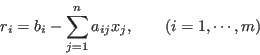
As in general no  can satisfy the equation system, there is always some
residual for each of the equations:
can satisfy the equation system, there is always some
residual for each of the equations:
or in matrix form
where
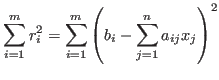
![${\bf r}=[r_1,\cdots,r_m]^T$](img711.png) . The total error can be defined as
. The total error can be defined as
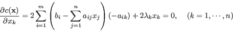
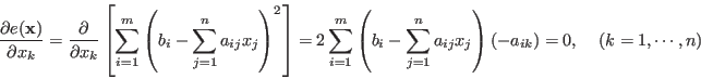
To find the optimal that minimizes  , we let
which yields
This can be expressed in the matrix form as
Or in matrix form we have:
Solving this for , we get the same result above. This matrix equation
can be solved for by multiplying both sides by the inverse of
 , if it exists:
where
is the pseudo-inverse of the non-square matrix  .
.
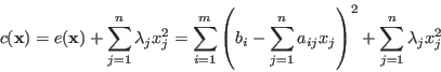
Sometime it is desired for the unknown  to be as small as possible, then
a cost function can be constructed as
to be as small as possible, then
a cost function can be constructed as
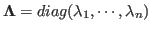
where a greater  means the size of the corresponding is more
tightly controlled. Then repeating the process above we get:
means the size of the corresponding is more
tightly controlled. Then repeating the process above we get:
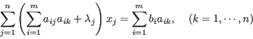
which yields
or in matrix form
where
 .
Solving this for we get:
.
Solving this for we get:
Next: Appendix
Up: algebra
Previous: Vector and matrix differentiation
Ruye Wang
2015-04-27
![\begin{displaymath}{\bf A}=\left[\begin{array}{ccc} a_{11} & \cdots & a_{1n}\\
...
...egin{array}{c}b_1 \vdots b_m\end{array}\right]_{m\times 1}
\end{displaymath}](img708.png)
![\begin{displaymath}\sum_{i=1}^m\sum_{j=1}^n a_{ij} a_{ik} x_j=\sum_{j=1}^n \left...
...ik}\right] x_j
=\sum_{i=1}^m b_i a_{ik},\;\;\;\;(k=1,\cdots,n) \end{displaymath}](img717.png)