Hopfield Network

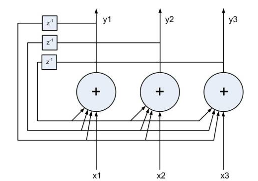
The Hopfield network has only a single layer of $n$ nodes. It behaves as an auto-associator (content addressable memory) with a set of $K$ n-D vector patterns $\{{\bf y}_k,\;\;k=1,\cdots,K\}$ stored in it. This is a supervised method which is first trained and then used as an auto-associator. This is a recurrent network, in the sense that the outputs of the nodes are fed back in an iterative process. When an incomplete or noisy version of one of the stored patterns is presented as the input, the complete pattern will be generated as the output after some iterations.

During the classification stage after the network is trained based on the Hebbian learning, the network can take an input pattern ${\bf x}_k$, a noisy or incomplete version of one of the pre-stored pattern:

$${\bf x}_k=[x_1^{(k)},\cdots, x_n^{(k)}]^T\;\;\;\;\;\;\;\;x_i \in\{-1,\;1\}$$

and responds to it by iteratively updating its output

$${\bf y}=[y_1,\cdots, y_n]^T\;\;\;\;\;\;\;\;\;\;y_i \in\{-1,\;1\}$$

until finally convergence is reached when one of the stored patterns which most closely resembles ${\bf x}$ is produced as the output.

Training:

The training process is essentially the same as the Hebbian learning, except here the two associated patterns in each pair are the same (self-association), i.e., ${\bf x}_k={\bf y}_k$, and the input and output patterns all have the same dimension $m=n$.

After the network is trained by Hebbian learning its weight matrix is obtained as the sum of the outer-products of the $K$ patterns to be stored:

$${\bf W}_{n\times n}=\frac{1}{n}\sum_{k=1}^K {\bf y}_k {\bf x}_k^T... ... \\ \vdots \\ y_n^{(k)} \end{array} \right] [ y_1^{(k)}, \cdots, y_n^{(k)} ]$$

the weight connecting node i and node j is

$$w_{ij}=\frac{1}{n}\sum_{k=1}^K y_i^{(k)} y_j^{(k)}=w_{ji}$$

We assume no self-connection exists $w_{ii}=0\;(i=1,\cdots,n)$

Classification:

When the weight matrix ${\bf W}$ is obtained by the training process, the network can be used to recognize an input pattern representing some noisy and incomplete version of one of those pre-stored patterns. When a pattern ${\bf x}$ is presented to the input nodes, the outputs nodes are updated iteratively and asynchronously. Only one of the $n$ nodes randomly selected is updated at a time:

$$x'_i=sgn \left(\sum_{j=1}^n w_{ij}x_j\right)=\left\{ \begin{array... ...geq 0 \\ -1, & \mbox{if}\;\;\;\sum_{j=1}^n w_{ij}x_j < 0 \end{array} \right.$$

where $x'_i=x_i(t_{n+1})$ represents the new output of the ith node while $x_i=x_i(t_n)$ represents the old one during the iteration. We now show that the iteration will always converge to produce one of the stored patterns as the output.

Energy function

We define the energy associated with a pair of nodes i and j as

$$e_{ij}\stackrel{\triangle}{=}-w_{ij}x_ix_j$$

and the interaction between these two nodes can be summarized by this table

$$\begin{tabular}{ r \vert r \vert\vert c \vert c} \hline $x_i$ & ... ... $e_{ij}<0$ \\ \hline 1 & 1 & $e_{ij}<0$ & $e_{ij}>0$ \\ \hline \end{tabular}$$

Two observations:

• Whenever the two nodes i and j are reinforcing each other's state, the energy $e_{ij}$ is negative. For example, in the first and last rows when $w_{ij}>0$, $x_i=\mp 1$ will help keep $x_j$ to stay at the same state $\mp 1$ in the iteration above, and the energy $e_{ij}<0$ is negative. Also in the two middle rows when $w_{ij}<0$, $x_i=\mp 1$ will help keep $x_j$ to stay at the same state $\pm 1$, and the energy $e_{ij}<0$ is negative.
• Whenever the two nodes i and j are trying to change each other's state, the energy is positive. For example, in the first and last rows when $w_{ij}<0$, $x_i=\mp 1$ will tend to reverse $x_j$ from its previous state $\mp 1$ to $\pm 1$, and the energy $e_{ij}>0$ is positive. Also in the two middle rows when $w_{ij}>0$, $x_i=\mp 1$ will tend to reverse $x_j$ from its previous state $\pm 1$ to $\mp 1$, and the energy $e_{ij}<0$ is positive.

In summary, low energy level of $e_{ij}$ corresponds to a stable interaction between $x_i$ and $x_j$, i.e., they tend to remain unchanged, and high energy level corresponds to an unstable interaction, i.e., they tend to change their states.

We next define the total energy function $E({\bf x})$ of all $n$ nodes in the network as the sum of all pair-wise energies:

$$E({\bf x}) \stackrel{\triangle}{=} \sum_{i>j} e_{ij}=-\sum_{i>j} \; w_{ij}x_ix_j =-\frac{1}{2}\sum_{i=1}^{n} \sum_{j=1}^{n} w_{ij} x_i x_j$$

Note that the last equation is due to $w_{ij}=w_{ji}$ and $w_{ii}=0$. Again, lower energy function level corresponds to more stable condition of the network, and vice versa.

The iteration and convergence

Now we show that the total energy $E({\bf x})$ always decreases whenever the state of any node changes. Assume $x_k$ has just been changeed, i.e., $x'_k \neq x_k$ ($x_k=\pm 1$ but $x'_k=\mp 1$), while all others remain the same $x'_{l \neq k} = x_{l \neq k}$. The energy before $x_k$ changes state is

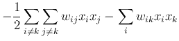
$$E({\bf x}) = -\frac{1}{2}[ \sum_{i\neq k}\sum_{j\neq k}w_{ij}x_ix_j + \sum_i w_{ik}x_ix_k + \sum_j w_{kj}x_kx_j ]$$

$$= -\frac{1}{2} \sum_{i\neq k}\sum_{j\neq k}w_{ij}x_ix_j - \sum_i w_{ik}x_ix_k$$

and the energy after $x_k$ changes state is

$$E'({\bf x})= -\frac{1}{2} \sum_{i\neq k}\sum_{j\neq k}w_{ij}x_ix_j - \sum_i w_{ik}x_ix'_k$$

The energy difference is

$$\bigtriangleup E = E'({\bf x})-E({\bf x}) =-(x'_k-x_k) \sum_i w_{ik}x_i=(x_k-x'_k) \sum_i w_{ik}x_i$$

Consider two cases:

• Case 1: if $x_k=-1$ but $\sum_i w_{ik}x_i \geq 0$, then $x'_k=1$, we have $(x_k-x'_k)=-2 \le 0$ and $\bigtriangleup E \leq 0$.
• Case 2: if $x_k=1$ but $\sum_i w_{ik}x_i < 0$, then $x'_k=-1$, we have $(x_k-x'_k)=2 \ge 0$ and $\bigtriangleup E \leq 0$.

As in either case, $\bigtriangleup E({\bf x}) \leq 0$ is always true throughout the iteration, and the magnitude of $E({\bf x})$ is finite, we conclude that the energy function $E({\bf x})$ will eventually reach one of the minima of the “energy landscape” and, therefore, the iteration will always converge.

Retrieval of stored patterns

Now we show the $K$ pre-stored patterns correspond to the minima of the energy function. First recall the weights of the network are obtained by Hebbian learning:

$$w_{ij}=\frac{1}{n}\sum_{k=1}^K y_i^{(k)} y_j^{(k)}$$

The energy function $E({\bf x})$ can be written as

$$E({\bf x}) = -\frac{1}{2}\sum_{i=1}^{n} \sum_{j=1}^{n} w_{ij} x_i x_j = -\frac... ...\frac{1}{2n}\sum_{k=1}^K \left[\sum_i \sum_j y_i^{(k)} x_i y_j^{(k)} x_j\right]$$

$$= -\frac{1}{2n}\sum_{k=1}^K \left[ \left(\sum_i y_i^{(k)} x_i\right... ...k)} x_i\right)^2 = -\frac{1}{2n}\sum_{k=1}^K \left({\bf y}_k^T {\bf x}\right)^2$$

If ${\bf x}$ is different from (ideally orthogonal to) any of the stored patterns, all $K$ terms of the summation will contribute to the sum only moderately (ideally if all patterns are orthogonal, all terms are zero). However, if ${\bf x}$ is the same as any one of the stored patterns, their inner product reaches maximum, causing the total energy to be minimized to reach one of the minima. In other words, the patterns stored in the net correspond to the local minima of the energy function. i.e., these patterns become attractors.

Note that it is possible to have other local minima, called spurious states, which do not represent any of the stored patterns, i.e., the associative memory is not perfect.