Hebb's Learning

Donald Hebb (Canadian Psychologist) speculated in 1949 that

“When neuron A repeatedly and persistently takes part in exciting neuron B, the synaptic connection from A to B will be strengthened.”

Simultaneous activation of neurons leads to pronounced increases in synaptic strength between them. In other words, "Neurons that fire together, wire together. Neurons that fire out of sync, fail to link". So a Hebbian network can be used as an associator which will establish the association between two sets of patterns $\{{\bf x}_k,\;\;k=1,\cdots,K \}$ and $\{{\bf y}_k,\;\;k=1,\cdots,K\}$.

The classical conditioning (Pavlov, 1927) could be explained by Hebbian learning:

• F: sight of food – unconditioned stimulus
• B: sound of bell – conditioned stimulus
• S: Salivation – response

$$(F \rightarrow S) \Rightarrow (F \cap B \rightarrow S) \Rightarrow (B \rightarrow S)$$

Synaptic connections between pattern B and pattern S are strengthened as both are repeatedly excited simultaneously.

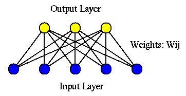
The structure

The Hebbian network is a supervised method with an input layer of $n$ nodes that take an input ${\bf x}=[x_1,\cdots,x_n]^T$ and an output layer of $m$ nodes that generate output ${\bf y}=[y_1,\cdots,y_m]^T$. Each output node $y_i$ is connected to each of the $n$ input nodes $x_j$ by a weight $w_{ij}$:

$$y_i=\sum_{j=1}^n w_{ij} x_j\;\;\;\;\;(i=1,\cdots,m)$$

In matrix form, we have

$${\bf y}_{m\times 1}={\bf W}_{m\times n}{\bf x}_{n\times 1}$$

The learning law

$$w_{ij}^{new}=w_{ij}^{old}+\eta x_j y_i\;\;\;\;(i=1,\cdots,m,\;j=1,\cdots,n)$$

or in matrix form:

$${\bf W}^{new}={\bf W}^{old}+\eta {\bf y} {\bf x}^T$$

Here $\eta$ is the learning rate, a parameter controlling how fast the weights are modified. The reasoning for this learning law is that when both $x_j$ and $y_i$ are high (activated), the weight $w_{ij}$ (synaptic connectivity) between them is enhanced according to Hebbian learning.

Training

If we assume $w_{ij}=0$ initially, $\eta=1$ and a set of $K$ pairs of patterns $\{ ({\bf x}_k,{\bf y}_k),\;\;k=1,\cdots,K \}$ are presented repeatedly in random order during training, we have

$$w_{ij}=\sum_{k=1}^Kx_j^{(k)}y_i^{(k)}\;\;\;\;(i=1,\cdots,m,\;\;j=1,\cdots,n)$$

or in matrix form, the weight matrix is the sum of the outer-products of all $K$ pairs of patterns:

$${\bf W}_{m\times n}=\sum_{k=1}^K {\bf y}_k {\bf x}_k^T = \sum_{k=... ... \\ \vdots \\ y_m^{(k)} \end{array} \right] [ x_1^{(k)}, \cdots, x_n^{(k)} ]$$

Classification

When presented with one of the patterns ${\bf x}_l$, the network will produce the output:

$${\bf y}={\bf W}{\bf x}_l=\left(\sum_{k=1}^K {\bf y}_k {\bf x}_k^T... ...={\bf y}_l({\bf x}_l^T{\bf x}_l)+\sum_{k\neq l}{\bf y}_k({\bf x}_k^T{\bf x}_l)$$

To interpret the output pattern ${\bf y}$, we first consider the ideal case where the following two conditions are satisfied:

• ${\bf x}$'s are orthogonal to each other:
  $${\bf x}_i^T{\bf x}_j=\vert{\bf x}_i\vert \vert{\bf x}_j\vert \cos... ...a_{ij}=\left\{ \begin{array}{ll} 1 & i=j \\ 0 & i\ne j \end{array} \right.$$
  where $\vert{\bf x}_i\vert$ is the length of vector ${\bf x}_i$ and $\phi$ is the angle between vectors ${\bf x}_i$ and ${\bf x}_j$.

  This condition implies that the $K$ input patterns are totally unrelated or uncorrelated to each other. How much two vectors are correlated to each other can be measured by the angular difference $\phi$ between them. If $\phi$ is close to 0, the two vectors are closely correlated, as their elements are very similar to each other so that they almost coincide. When negative values are allowed for the elements and $\phi$ is close to 180 degrees, the vectors are also highly correlated as their elements are opposite to each other. In either case, $\cos \phi$ is close to 1 and the inner product is maximized, indicating that the two vectors are either positively or negatively related to each other. On the other hand, if the two vectors are perpendicular to each other ( $\phi=\pm 90^\circ$, $\cos \phi = 0$), the inner product of the two vectors is zero, indicating the elements of the two vectors are irrelevant to those of the other.

  How much two patterns ${\bf x}_i$ and ${\bf x}_j$ are related to each other can also be measured quantitatively, we define correlation coefficient as:

  $$r_{ij}\stackrel{\triangle}{=}\frac{{\bf x}_i^T{\bf x}_j}{\vert\ve... ... =\frac{\sum_k x_{ik} x_{jk}}{\sqrt{\sum_k x_{ik}^2}\sqrt{\sum_k y_{jk}^2} }$$
  $r_{ij}$ is the inner product of two normalized vectors representing two patterns in the n-D feature space, and can take the following values
  • $0 < r_{ij} \leq 1$, if ${\bf x}_i$ and ${\bf x}_j$ are positively correlated ($r_{ij}=1$ iff ${\bf x}_i={\bf x}_j$)
  • $r_{ij} =0$, if ${\bf x}_i$ and ${\bf x}_j$ are not correlated
  • $-1<r_{ij} \leq 0$, if ${\bf x}_i$ and ${\bf x}_j$ are negatively correlated ($r_{ij}=-1$ iff ${\bf x}_i=-{\bf x}_j$)

  In other words, if ${\bf x}_i$ and ${\bf x}_j$ are totally uncorrelated, then $r_{ij} =0$ and they are orthogonal to each other.

• The number of pattern pairs is smaller than the number of dimensions (the number of input nodes): $K \leq n$. This condition implies that the capacity of the network ($n$ input nodes) is large enough for representing $K$ different patterns. In mathematical terms, there can be no more than $n$ orthogonal vectors in an n-D space.

If these conditions are true, then the response of the network to ${\bf x}_l$ will be

$${\bf y}={\bf y}_l({\bf x}_l^T{\bf x}_l)+\sum_{k\neq l}{\bf y}_k({\bf x}_k^T{\bf x}_l)={\bf y}_l$$

because all other terms are zero: ${\bf x}_k^T {\bf x}_l=0,\;\;(k \ne l)$. In other words, a one-to-one correspondence relationship between ${\bf x}_k$ and ${\bf y}_k$ has been established for all $k=1,\cdots,K$. In non-ideal cases, the summation term (called cross talk) is non-zero and we have an error $\vert\vert{\bf y}-{\bf y}_l\vert\vert > 0$.

Although two patterns ${\bf x}=B$ and ${\bf y}=S$ don't have causal relationship (as $S$ is caused by another pattern $F$), if they always appear simultaneously, an association relationship can be established in the Hebbian network.