Self-Organizing Map (SOM)

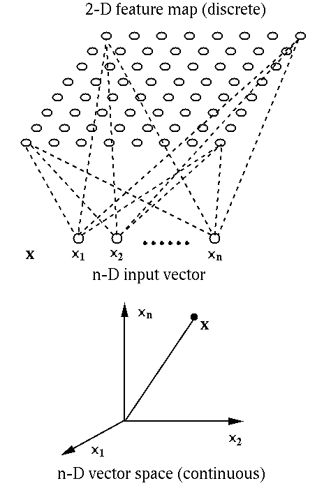
Self-organizing map (SOM), also referred to as self-organized feature mapping (SOFM) (by Finnish professor Teuvo Kohonen) is a process that maps the input patterns in a high-dimensional vector space to a low-dimensional (typically 2-D) output space, the feature map, so that the nodes in the neighborhood of this map respond similarly to a group of similar input patterns. The idea of SOM is motivated by the mapping process in the brain, by which signals from various sensory (e.g., visual and auditory) system are projected (mapped) to different 2-D cortical areas and responded to by the neurons wherein.

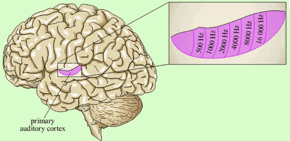
For example, sound signals of different frequencies are mapped to the primary auditory cortex in which neighboring neurons respond to similar frequencies.

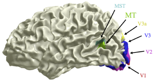
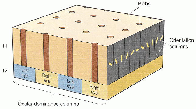
Similarly, due to the retinotopic mapping in the visual system, the visual signals received by the retina are topographically mapped to the primary and then subsequent higher visual cortical areas. For example, the visual edges/lines of different orientations are also mapped to the primary visual cortex where neighboring neurons respond to similar orientations.

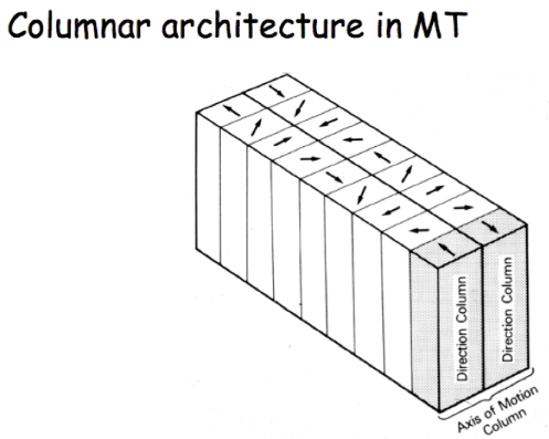
All examples above show a common characteristic of some biological neural networks, the neurons are spatially organized in such a way that nearby neurons respond to similar patterns. The SOM network mimics this property.

The output nodes of a SOM network are typically organized in a low-dimensional (typically 2-D array, although 1-D and 3-D can also be used), a lattice or a grid, and the competitive learning algorithm discussed above is modified so that the learning takes place not only at the winning node $y_k$, but also at a set of output nodes $y_i$ in the neighborhood of the winning node in the 2-D output space:

$${\bf w}_i^{new}={\bf w}_i^{old}+u_{ik}\triangle {\bf w}_i^{old} ={\bf w}_i^{old}+u_{ik}\eta ({\bf x}-{\bf w}_i^{old}),\;\;\;\;\;\;i=1,\cdots,m$$

where $u_{ik}$ is some weighting function centered at the winning node. For example,

$$u_{ik}=\left\{\begin{array}{ll} 1 & d_{ik}< T\\ 0 & \mbox{otherwise} \end{array}\right.$$

where $d_{ik}$ is the Euclidean distance between node $y_i$ and the winning node $y_k$ in the 2-D output space, and $T$ is a pre-set threshold value. Alternatively, $u_{ik}$ can be a Gaussian function:

$$u_{ik}=exp\left(-\frac{d^2_{ik}}{2\sigma^2}\right)$$

where $\sigma$ is a parameter for the width of the Gaussian function. We see that in this cases, learning takes place for all $m$ output nodes as they all get to update their weights. But those nodes closer to the input vector will learn more than those that are farther away.

A slightly different weighting function can be used. In each iteration of the competitive learning process, we first sort all distances $d_i=\vert\vert{\bf x}-{\bf w}_i\vert\vert$ for all $i=1,\cdots,m$ so that

$$d_{i_0}\le d_{i_1}\le \cdots \le d_{i_m}$$

and then use the learning rule:

$${\bf w}_{i_k}^{new}={\bf w}_{i_k}^{old}+e^{-k/\sigma}\eta ({\bf x}-{\bf w}_{i_k}^{old}), \;\;\;\;\;\;(k=1,\cdots,m)$$

The network with this learning rule is called neural gas.

Here are the steps of the SOM learning algorithm:

1. Arrange a set of output nodes with random weights in a low dimensional grid (1-D, 2-D, or 3-D).
2. Choose a random input pattern from the high-dimensional feature space and calculate the activations for each of the output nodes
3. Find the winning node $y_k$ and update the weights of all nodes in its neighborhood
4. Go back to step 2 until the feature map is no longer changing or a set maximum number of iterations is reached.

In the training process, both the size of the neighborhood ($T$ or $\sigma$) and the learning rate $\eta$ will gradually reduce.

We see that the SOM is a discrete approximation of the patterns defined in a continuous n-D feature space, i.e., the uncountably infinite number of possible patterns are quantified and approximated by a finite set of n-D vectors each represented by an output node in the 2-D grid. Also, as the nodes in the 2-D grid are spatially related, they present a visualization of the clustering structure of the high-dimensional data. Therefore the most important applications of the SOM are in the visualization of high-dimensional systems and processes and discovery of categories and abstractions from raw data.

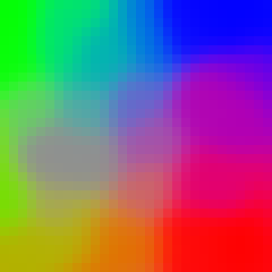
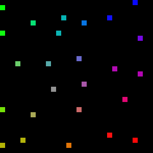
Example 0:

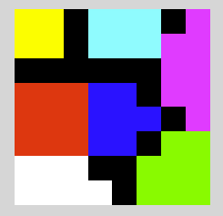
A set of different colors can be treated as vectors in a 3-D vector space. We can train a SOM network so that the nodes in the 2-D output layer self organizes to form a map that responds to different colors (left) as well as the specific input vectors used in the training (right).

List below are some other applications of the SOM netowrk:

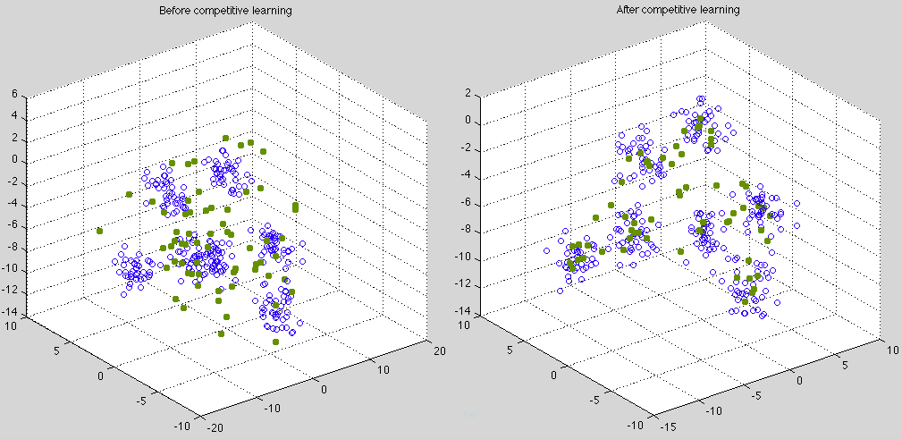
Example 0:

The $C=7$ clusters of $N=4$ dimensional data points and the weight vectors projected to a 3-D space by PCA transform, before (left) and after (right) the competitive learning.

The figure below is the 2-D SOM formed by the output nodes after learning. Note that the neighobring nodes have learned to respond to similar input vectors belonging to the same cluster (with same color coding). The black areas represent those output nodes not responding to any of the inputs (their weight vectors are represented by the red dots in between the clusters in the previous figure on the right).

Example 1: 2-D SOM trained by a set of random dots:

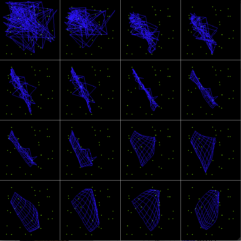
The first 16 iterations

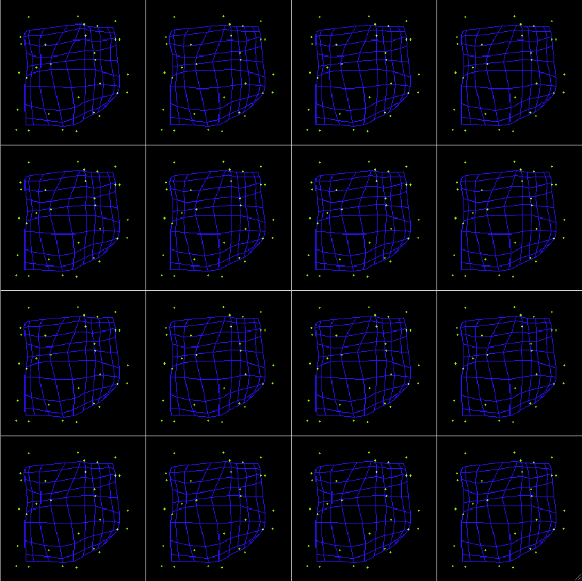
The last 16 iterations

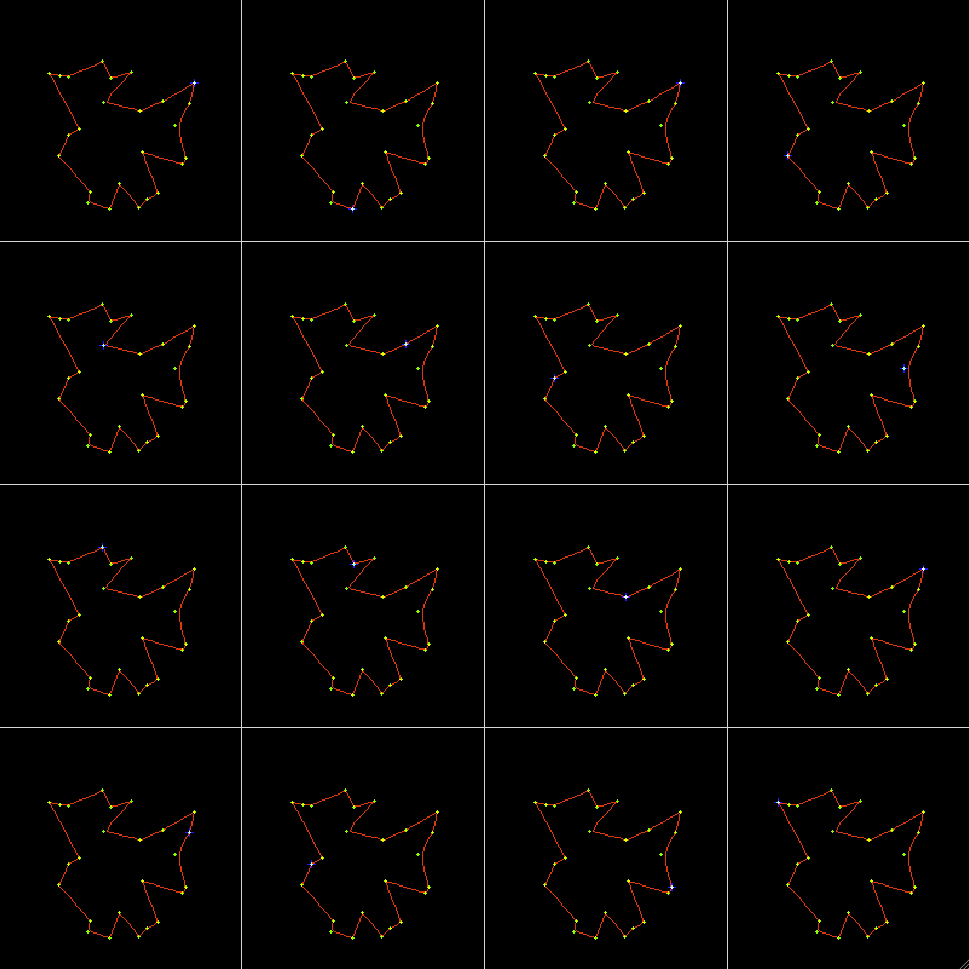
Example 2: Traveling salesman problem, 1-D SOM trained by a set of random dots:

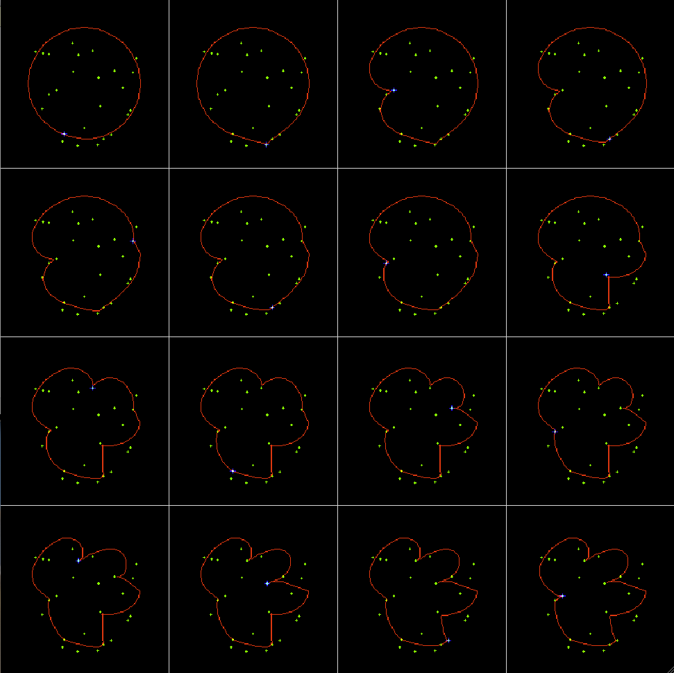
The first 16 iterations

The last 16 iterations