Radial-Basis Function (RBF) Networks

The radial basis function (RBF) networks are inspired by biological neural systems, in which neurons are organized hierarchically in various pathways for signal processing, and they are tuned to respond selectively to different features/characteristics of the stimuli within their respective fields. In general, neurons in higher layers have larger receptive fields and they selectively respond to more global and complex patterns.

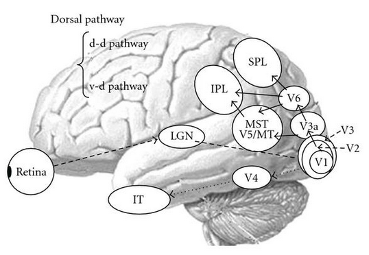
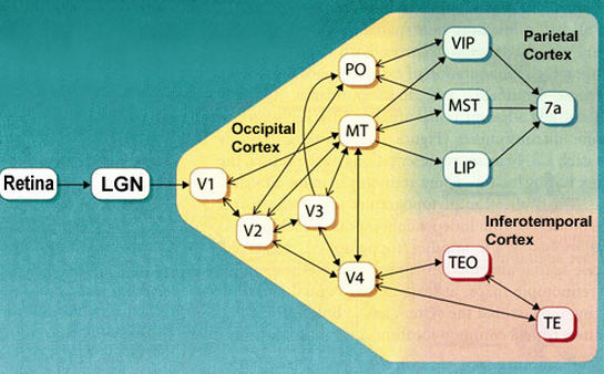
For example, neurons at different levels along the visual pathway respond selectively to different types of visual stimuli:

• Neurons in the primary visual cortex (V1) receive visual input from the retina and selectively respond to different orientations of linear features;
• Neurons in the middle temporal (MT) area receive visual input from the V1 area and selectively respond to different motion directions;
• Neurons in the medial superior temporal area (MST) receive visual input from the MT area and selectively respond to different motion patterns (optic flow) such as rotation, expansion, contraction, and spiral motions.

Moreover, neurons in the auditory cortex respond selectively to different frequencies.

The tuning curves, the local response functions, of these neurons are typically Gaussian, i.e., the level of response is reduced when the stimulus becomes less similar to what the cell is most sensitive and responsive to (the most preferred).

These Gaussian-like functions can also be treated as a set of basis functions (not necessarily orthogonal and over-complete) that span the space of all input patters. Based on such local features represented by the nodes, a node in a higher layer can be trained to selectively so that it is specialized to respond to some specific patterns/objects (e.g., “grandmother cell”), based on the outputs of the nodes in the lower layer.

Applications:

• The RBF network can be used in pattern classification, by which a given pattern vector ${\bf x}$ is classified into one of classes. The classification is typically supervised, i.e., the network is trained based on a set of $K$ training patterns $( \omega_k, {\bf x}_k)$ ($k=1,\cdots,K$), where $\omega_k$ indicates the class the kth pattern ${\bf x}_k$ belongs, i.e., ${\bf x}_k\in\omega_k$.

  

• RBF networks can also be used for non-parametric regression. In parametric regression, the form of the function of interest is known, such as linear regression, $y=f(x)=ax+b$. All we need to do is to find a set of parameters, e.g., $a$ and $b$, based on the observed data $(y_k, x_k)$ ($k=1,\cdots,K$). However, in non-parametric regression, little knowledge is available regarding the type and form of the function $y=f(x)$. For example, in time-series predicting, the value $y_k=x(t_k)$ of a time series can be estimated/predicted from the $N$ previous values ${\bf x}_k=[x(t_{k-1}),\;x(t_{k-2}),\cdots,x(t_{k-N})]^T$ based on $K$ observations $(y_k,{\bf x}_k)$ ($k=1,\cdots,K$). This problem can also be viewed as fitting a hyper-surface $\hat{y}=f({\bf x})$ in an N-dimensional space to a set of $K$ data points $\{ (y_k, {\bf x}_k),\;k=1,\cdots,K \}$.

  

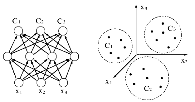
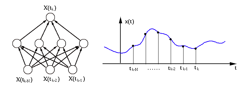
As seen in the examples above, an RBF network is typically composed of three layers, the input layer composed of $N$ nodes that receive the input signal ${\bf x}$, the hidden layer composed of $L$ nodes that simulate the neurons with selective tuning to different features in the input, and the output layer composed of $M$ nodes simulating the neurons at some higher level that respond to features at a more global level, based on the output from the hidden layer representing different features at a local level. (This could be considered as a model for the visual signal processing in the pathway $retina \Rightarrow V1 \Rightarrow MT \Rightarrow MST$.)

Upon receiving an input pattern vector ${\bf x}$, the jth hidden node reaches the activation level:

$$h_j({\bf x})=exp[-({\bf x}-{\bf c}_j)^T {\bf\Sigma}_j^{-1}({\bf x}-{\bf c}_j)]$$

where ${\bf c}_j$ and ${\bf\Sigma}_j$ are respectively the mean vector and covariance matrix associated with the jth hidden node. In particular, the covariance matrix is a special diagonal matrix ${\bf\Sigma}=\sigma^2{\bf I}=diag(\cdots, \sigma^2,\cdots)$, then the Gaussian function becomes isotropic and we have

$$h_j({\bf x})=exp[-({\bf x}-{\bf c}_j)^2/\sigma^2]$$

We see that ${\bf c}_j$ represents the preferred feature (orientation, motion direction, frequency, etc.) of the jth neuron. When ${\bf x}={\bf c}_j$, the response of the neuron is maximized due to the selectivity of the neuron.

In the output layer, each node receives the outputs of all nodes in the hidden layer, and the output of the ith output node is the linear combination of the net activation:

$$f_i({\bf x})=\sum_{j=1}^L w_{ij} h_j({\bf x}) =\sum_{j=1}^L w_{ij}\; exp[-({\bf x}-{\bf c}_j)^T {\bf\Sigma}_j^{-1}({\bf x}-{\bf c}_j)]$$

Note that the computation at the hidden layer is non-linear but that at the output layer is linear, i.e., this is a hybrid training scheme.

Learning Rules

Through the training stage, various system parameters of an RBF network will be obtained, including the ${\bf c}_j$ and ${\bf\Sigma}_j$ ($j=1,\cdots,L$) of the $L$ nodes of the hidden layer, as well as the weights $w_{ij}$ ( $j=1,\cdots,L,\;\;i=1,\cdots,M$) for the $M$ nodes of the output layer, each fully connected to all $L$ hidden nodes.

• Training of the hidden layer

  The centers ${\bf c}_j$ ($j=1,\cdots,L$) of the $L$ nodes of the hidden layer can be obtained in different ways, so long as the entire data space can be well represented.

  • They can be chosen randomly from the input data set ${\bf x}_k$ ( $k=1,\cdots,K$).
  • The centers can be obtained by unsupervised learning (SOM, k-means clustering) based on the training data.
  • The covariance matrix ${\bf\Sigma}_j$ as well as the center ${\bf c}_j$ can also be obtained by supervised learning.

• Training of the output layer

  Once the parameters ${\bf c}_j$ and ${\bf\Sigma}_j$ are available, we can concentrate on finding the weights $w_j$ of the output layer, based on the given training data containing $K$ data points $\{ y_k, {\bf x}_k\; (k=1,\cdots,K)\}$, i.e., we need to solve the equation system for the $L$ weights $w_j$ ($j=1,\cdots,L$):

  $$y_k=f({\bf x}_k)=\sum_{j=1}^L w_j h_j({\bf x}_k),\;\;\;\;\;\;(k=1,\cdots,K)$$
  This equation system can also be expressed in matrix form:
  $${\bf y}={\bf H}{\bf w}$$
  where ${\bf y}=[y_1,\cdots,y_K]^T$, ${\bf w}=[w_1,\cdots w_L]^T$, and ${\bf H}$ is an $K \times L$ matrix function of the $K$ input vectors ${\bf x}_k$:
  $${\bf H}=\left[\begin{array}{ccc}h_1({\bf x}_1)&\cdots&h_1({\bf x}... ...dots \\ h_L({\bf x}_1)&\cdots&h_L({\bf x}_K) \end{array}\right]_{L\times K}$$
  As the number of training data pairs $K$ is typically much greater than the number of hidden nodes $L$, the equation system above contains more equations than unknowns, and has no solution. However, we can still try to find an optimal solution so that the actual output $\hat{{\bf y}} ={\bf H}{\bf w}$ approximates ${\bf y}$ with a minimal mean squared error (MSE):
  $$MSE=\vert\vert{\bf y}-\hat{\bf y}\vert\vert^2=\vert\vert{\bf y}-{... ...x}_k) ]^2 =\sum_{k=1}^K \left[y_k-\sum_{j=1}^L w_j h_j({\bf x}_k)\right]^2$$
  To find the weights as the parameters of the model, the general linear least squares can be used, based on the pseudo inverse of the non-square matrix:
  $${\bf w}=({\bf H}^T{\bf H})^{-1}{\bf H}^T {\bf y}={\bf H}^-{\bf y}$$

  In some cases (e.g., for the model of $x(t)$ to be smooth), it is desirable for the weights to be small. To achieve this goal, a cost function can be constructed with an additional term added to the MSE:

  $$\vert\vert{\bf y}-\hat{{\bf y}}\vert\vert^2+\lambda \vert\vert{\bf w}\vert\vert^2$$
  As shown in Appendix B, the optimal solution of this system is
  $${\bf w}=({\bf H}^T{\bf H}+\lambda {\bf I})^{-1}{\bf H}^T {\bf y}$$