Covariance and Correlation

In principal component analysis (PCA), each pattern ${\bf x}$ is treated as a random vector of which each component $x_i$ is a random variable with mean and variance

$$\mu_i = E[ {\bf x}_i ]=\int x_i\, p(x_i)\, dx_i$$

$$\sigma_i^2 = E[ (x_i-\mu_i)^2 ]=E[x_i^2]-\mu_i^2 =\int x_i^2\,p(x_i)\, dx_i-\mu_{x_i}^2,\;\;\;\; (i=1,\cdots,d)$$ (37)

and the covariance of $x_i$ and $x_j$ is:

$$\sigma_{ij}^2 = E[ (x_i-\mu_i)(x_j-\mu_j) ]=E[ x_ix_j ]-\mu_i\mu_j$$

$$= \int\int x_i x_j\,p(x_i,x_j)\,dx_i\,dx_j-\mu_i\mu_j \;\;\;\;\;\;\;(i,j=1,\cdots,d)$$ (38)

then the mean vector and covariance matrix of ${\bf x}$ are:

$${\bf m}_x = E[ {\bf x} ]=\left[\begin{array}{c} \mu_1\\ \vdots\\ \mu_d\end{array}\right]$$

$${\bf\Sigma}_x = E[ ({\bf x}-{\bf m}_x)({\bf x}-{\bf m}_x)^T ] =E[ {\bf xx}^T ]-{\... ... & \ddots & \vdots \\ \sigma_{d1}^2 & \cdots & \sigma_{dd}^2\end{array}\right]$$ (39)

Usually the joint probability density function $p({\bf x})=p(x_1,\cdots,x_d)$ of the random vector ${\bf x}$ is unknown. In this case, the mean vector ${\bf m}_x$ and covariance matrix ${\bf\Sigma}_x$ of ${\bf x}$ can be estimated by the method of maximum likelihood estimation (MLE) based on a set of observed data samples ${\bf X}=[{\bf x}_1,\cdots,{\bf x}_N]$:

$$\hat{\bf m}_x=\frac{1}{N}\sum_{n=1}^N {\bf x}_n,\;\;\;\;\;\;\;\; ... ...bf m})^T =\frac{1}{N}\sum_{n=1}^N {\bf x}_n{\bf x}_n^T-\hat{\bf m}\hat{\bf m}^T$$ (40)

Note that the rank of the $d \times d$ estimated covariance matrix $\hat{\bf\Sigma}$ is at most $N-1$, due to the $N$ samples in the dataset ${\bf X}$, assumed to be are independent, and the additional constraint:

$$\sum_{n=1}^N({\bf x}_n-\hat{\bf m})=\sum_{n=1}^N{\bf x}_n-N\hat{\bf m}={\bf0}$$ (41)

The variance $\sigma_i^2=E[(x_i-\mu_{x_i})^2]$ can be treated as the dynamic energy contained in $x_i$, or the amount of information carried by $x_i$, while the trace $tr{\bf\Sigma}_x=\sum_{i=1}^d\sigma_i^2$ can be considered as the total amount of dynamic energy contained in ${\bf x}$. Also, the covariance $\sigma_{ij}^2=E[(x_i-\mu_{x_i})(x_j-\mu_{x_j})]$ can be considered as the mutual energy, a measure of the correlation between $x_i$ and $x_j$. By normalizing the covariance $\sigma_{ij}^2$, we get the correlation coefficient between $x_i$ and $x_j$:

$$r_{ij}=\frac{\sigma_{ij}^2 }{\sqrt{ \sigma_i^2\;\sigma_j^2}} =\frac{\sigma_{ij}^2}{ \sigma_i\;\sigma_j}$$ (42)

that measures how the two random variables $x_i$ and $x_j$ are correlated.

• $r_{ij}=\pm 1$ or $\vert r_{ij}\vert=1$: $x_i$ and $x_j$ are maximally correlated. The information contained in the two variables is completely redendant, given the value of one of them, the value of the other is known.

• $-1<r_{ij}<1$ or $\vert r_{ij}\vert<1$: $x_i$ and $x_j$ are correlated to different extents. The information they each carry has certain redendancy.

• $r_{ij}=0$: $x_i$ and $x_j$ are uncorrelated. They each carry their own independent information with no redencdancy.

We see that the orrelation coefficient $r_{ij}$ that measures how much two random variables are correlated also measures the redendancy of the information they carry. When there exists some data redendancy in the data, it is possible to carry out data compression by some method such as the principal component analysis based on the covariance ${\bf\Sigma}$ to reduce the data redendancy, so that the data size can be significantly reduced while the information (dynamic energy) contained in the data is still mostly preserved.

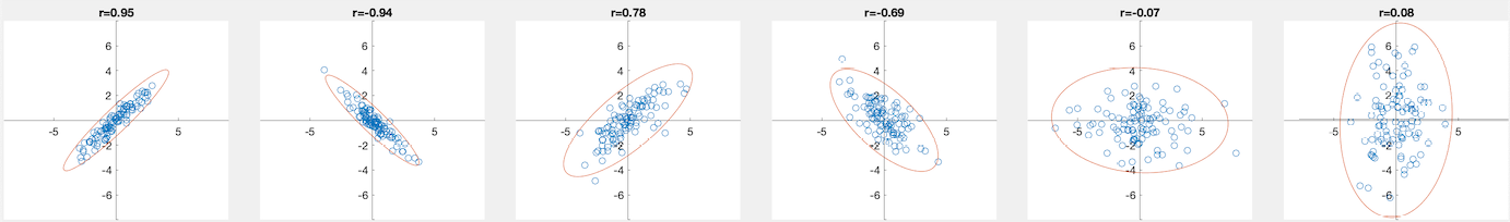
Examples

Six normally distributed 2-D datasets are generated with zero mean and the following covariance matrices:

$${\bf\Sigma}_1=\left[\begin{array}{rr} 1.0 & 0.95 \\ 0.95 & 1\end{... ...\Sigma}_3=\left[\begin{array}{rr} 1 & 0 \\ 0 & 3\end{array}\right],\;\;\;\;\;\;$$ (43)

These data points are plotted below, together with the correlation coefficient on top of each dataset.