Kernel PCA

In kernel PCA, the PCA method, which maps the dataset to a low dimensional space, and the kernel method, which maps the datad set to a high dimensional space, are combined to take advantage of both the high dimensional space (e.g., better separability) and the low dimensional space (e.g., computational efficiency).

Specifically, we assume the given dataset ${\bf X}=[{\bf x}_1,\cdots,{\bf x}_N]$ in the original d-dimensional feature space is mapped into ${\bf Z}=[{\bf z}_1,\cdots,{\bf z}_N]$ in a high dimensional space. Correspoindingly, the inner product ${\bf x}_m^T{\bf x}_n$ in the original space is mapped into an inner product in the high dimensional space:

$${\bf z}_m^T{\bf z}_n=K({\bf x}_m,{\bf x}_n)=k_{mn} \;\;\;\;\;\;\;(m,n=1,\cdots,N)$$ (108)

Given $N$ data points in the dataset ${\bf X}$, we can further define a kernel matrix:

$${\bf K}={\bf Z}^T{\bf Z} =\left[\begin{array}{c}{\bf z}_1^T\\ \vd... ...&\cdots&k_{1N}\\ \vdots&\ddots&\vdots\\ k_{N1}&\cdots&k_{NN}\end{array}\right]$$ (109)

To carry out KLT in the high dimensional space, we need to estimate the covariance matrix of ${\bf z}=\phi({\bf x})$:

$${\bf\Sigma}_z =\frac{1}{N}\sum_{n=1}^N ({\bf z}_n-{\bf m}_z)({\bf... ...\bf m}_z)^T =\frac{1}{N}\sum_{n=1}^N {\bf z}_n{\bf z}_n^T -{\bf m}_z{\bf m}_z^T$$ (110)

We first assume the samples in ${\bf Z}=[{\bf z}_1,\cdots,{\bf z}_N]$ have a zero mean ${\bf m}_z={\bf0}$, which will be justified later, and get (same as Eq. (82)):

$${\bf\Sigma}_z =\frac{1}{N}\sum_{n=1}^N ({\bf z}_n-{\bf m}_z)({\bf... ...{c} {\bf z}_1^T\\ \vdots\\ {\bf z}_N^T\end{array}\right] =\frac{1}{N}{\bf ZZ}^T$$ (111)

and its eigenequations:

$${\bf\Sigma}_z{\bf v}_n=\left(\frac{1}{N}{\bf ZZ}^T\right){\bf v}_n =\lambda_n{\bf v}_n\;\;\;\;\;\;\; (n=1,2,\cdots)$$ (112)

We then premultiply ${\bf Z}^T$ on both sides of the eigenequation above to get (same as Eq. (83)):

$$\frac{1}{N}{\bf Z}^T{\bf Z}\left({\bf Z}^T{\bf v}_n\right) =\frac{1}{N}{\bf K u}_n =\lambda_n\left({\bf Z}^T{\bf v}_n\right)=\lambda_n{\bf u}_n$$ (113)

where ${\bf u}_n={\bf Z}^T{\bf v}_n$. Solving this eigenequation of the $N\times N$ matrix ${\bf Z}^T{\bf Z}/N={\bf K}/N$, we get its eigenvectors ${\bf u}_n={\bf Z}^T{\bf v}_n\;(n=1,\cdots,N)$, corresponding to the eigenvalues $\{\lambda_1,\cdots,\lambda_N\}$, which are the same as the non-zero eigenvalues of ${\bf\Sigma}_z={\bf ZZ}^T/N$. The eigenvectors ${\bf v}_n$ of ${\bf\Sigma}_z$ in Eq. (112) can now be written as:

$${\bf v}_n=\frac{1}{\lambda_nN}{\bf Z}\left({\bf Z}^T{\bf v}_n\right) =\frac{1}{\lambda_n N}{\bf Z}{\bf u}_n$$ (114)

which can be further normalized by imposing the condition $\vert\vert{\bf v}_n\vert\vert^2=1$:

$$\vert\vert{\bf v}_n\vert\vert^2 = {\bf v}_n^T{\bf v}_n =\frac{1}{(\lambda_n N)^2}({\bf Zu}_n)^T({\bf Zu}_n) =\frac{1}{(\lambda_n N)^2}{\bf u}_n^T{\bf Z}^T{\bf Zu}_n$$

$$= \frac{1}{(\lambda_n N)^2}{\bf u}_n^T{\bf K}{\bf u}_n =\frac{1}{\l... ... N}{\bf u}_n^T{\bf u}_n =\frac{1}{\lambda_n N}\vert\vert{\bf u}_n\vert\vert^2=1$$ (115)

We see that if the eigenvectors ${\bf u}_n$ of ${\bf K}$ are rescaled to satisfy $\vert\vert{\bf u}_n\vert\vert^2=\lambda_n N$, then the eigenvectors ${\bf v}_n$ of ${\bf\Sigma}_z$ are normalized to satisfy $\vert\vert{\bf v}_n\vert\vert^2=1$. Now we can carry out PCA in the high dimensional space by

$${\bf y}=[{\bf v}_1,\cdots,{\bf v}_N]^T{\bf z}={\bf V}^T{\bf z}$$ (116)

of which each component $y_n={\bf v}^T{\bf z}$ is the projection of ${\bf z}=\phi({\bf x})$ onto one of the eigenvectors ${\bf v}_n$ of ${\bf\Sigma}_z$:

$$y_n={\bf z}^T{\bf v}_n = {\bf z}^T\left(\frac{1}{\lambda_n N}{\bf Z}{\bf u}_n \right) =\fr... ...{\bf u}_n =\frac{1}{\lambda_n N}{\bf z}^T[{\bf z}_1,\cdots,{\bf z}_N] {\bf u}_n$$

$$= \frac{1}{\lambda_n N}[{\bf z}^T{\bf z}_1,\cdots,{\bf z}^T{\bf z}_... ...bf u}_n =\frac{1}{\lambda_n N}{\bf k}^T{\bf u}_n,\;\;\;\;\;\;\;\;(n=1,\cdots,N)$$ (117)

where we have defined $k_n={\bf z}^T{\bf z}_n$ and ${\bf k}=[k_1,\cdots,k_N]^T$. Although neither ${\bf z}$ nor ${\bf v}_n={\bf Zu}_n/\lambda_nN$ is available, their inner product $y_n={\bf z}^T{\bf v}_n$ can still be obtained based on the kernel function $k_n={\bf z}^T{\bf z}_n$. We see that all data points in the high dimensional space appear only in the form of an inner product in the equation above, as well as in the eigenequation Eq. (113), the kernel mapping ${\bf z}=\phi({\bf x})$ never needs to be explicitly carried out.

The discussion above is based on the assumption that the data in the high dimensional space have zero mean ${\bf m}_z={\bf0}$. This cannot be achived by subtracting the mean from the data to get $\tilde{\bf z}={\bf z}-{\bf m}_z$, as neither ${\bf z}$ nor ${\bf m}_z$ is available without carrying out the kernel mapping ${\bf z}=\phi({\bf x})$. However, we can find the inner product of two zero-mean data points in the high dimensional space as

$$\tilde{k}_{mn} = \tilde{\bf z}_m^T\tilde{\bf z}_n =({\bf z}_m-{\bf m}_z)^T({\bf z}... ...}^N {\bf z}_k\right)^T \left({\bf z}_n-\frac{1}{N}\sum_{l=1}^N {\bf z}_l\right)$$

$$= {\bf z}_m^T{\bf z}_n -{\bf z}_m^T\left(\frac{1}{N}\sum_{l=1}^N {\... ...T\right) {\bf z}_n +\frac{1}{N^2}\sum_{k=1}^N\sum_{l=1}^N {\bf z}_k^T {\bf z}_l$$

$$= k_{mn}-\frac{1}{N}\sum_{l=1}^N k_{ml}-\frac{1}{N}\sum_{k=1}^N k_{kn} +\frac{1}{N^2}\sum_{k=1}^K\sum_{l=1}^N k_{kl},\;\;\;\;\;\;\;(m,n=1,\cdots,N)$$ (118)

The kernel matrix composed of all $N\times N$ such inner products can be written as:

$$\tilde{\bf K}={\bf K}-{\bf 1}_N{\bf K}-{\bf K}{\bf 1}_N+{\bf 1}_N{\bf K1}_N$$ (119)

where

$${\bf 1}_N=\frac{1}{N}\left[\begin{array}{ccc} 1&\cdots&1\\ \vdots&\ddots&\vdots\\ 1&\cdots&1\end{array}\right]_{N\times N}$$ (120)

If we replace the kernel matrix ${\bf K}$ for ${\bf z}$ with non-zero mean in the algorithm considered above by $\tilde{\bf K}$ for $\tilde{\bf z}$ with zero mean, then the assumption that ${\bf z}$ has zero mean ${\bf m}_z$ becomes valid. In summary, here are the steps of the kernel PCA algorithm:

• Given the dataset ${\bf X}=\{ {\bf x}_1,\cdots,{\bf x}_N\}$, obtain ${\bf K}$ based on kernel mapping $k_{mn}=k({\bf x}_m,{\bf x}_n)$ for all $m,n=1,\cdots,N$, and then find $\tilde{\bf K}$, as in Eq. (119);
• Solve eigenvalue problem of $\tilde{\bf K}$ to get the eigenvalue $\lambda_n$ and the corresponding eigenvector ${\bf u}_n$ for all $i=1,\cdots,N$;
• Project each data point ${\bf z}=\phi({\bf x})$ (implicit) onto the nth eigenvector ${\bf v}_n$ to get the principal component: $y_n={\bf z}^T{\bf v}_n={\bf k}^T{\bf u}_n/\lambda_n N$ for each $n=1,\cdots,N$, as in Eq. (117).
• Carry out whatever operation (e.g., feature selection, classification) in the subspace spanned by the first $M<N$ principal components $\{y_1,\cdots,y_M\}$ in the high dimensional feature space, containing most of the information.

Note that in kernel PCA methods, the complexity for solving the eigenvalue problem of the $N\times N$ kernel matrix ${\bf K}$ is $O(N^3)$, instead of $O(d^3)$ for the linear PCA based on the $d \times d$ covariance matrix ${\bf\Sigma}_x$.

Shown below is a Matlab function for the kernel PCA algorithm which takes the dataset ${\bf X}=[{\bf x}_1,\cdots,{\bf x}_N]$ as input and generates the eigenvalues in ${\bf d}$ and the dataset in the transform space ${\bf Y}$. The function Kernel(X,X) calculates the kernel matrix ${\bf K}$.

function [Y d]=KPCA(X)
    [D N]=size(X);
    K=Kernel(X,X);                      % kernel matrix of data X
    one=ones(N)/N;    
    Kt=K-one*K-K*one+one*K*one;         % Kernel matrix of data with zero mean
    [U D]=eig(Kt);                      % solve eigenvalue problem for K
    [d idx]=sort(diag(D),'descend');    % sort eigenvalues in descending order
    U=U(:,idx);
    D=D(:,idx);
    for n=1:N
        U(:,n)=U(:,n)/d(n)/N;
    end
    Y=(K*U)';   
end

Examples:

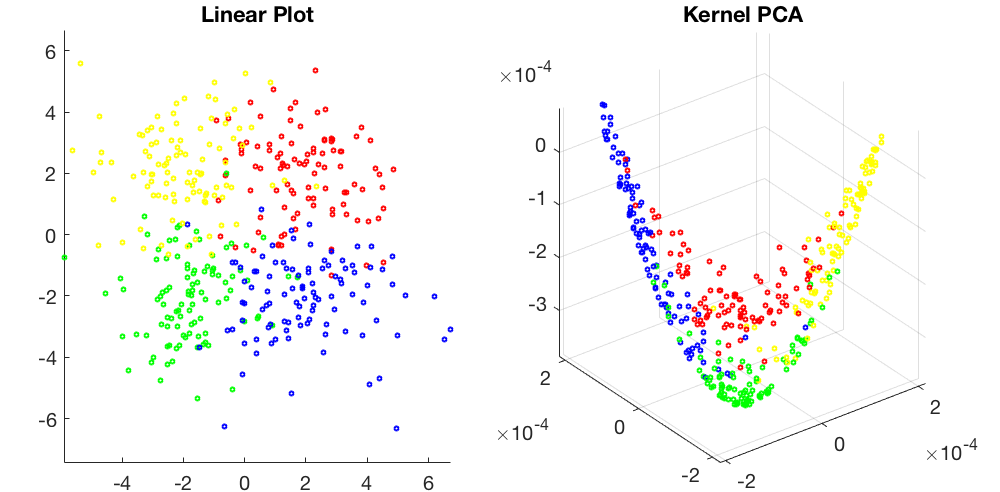
Visualization of a 2-D dataset of four classes, linear plot on the left and kernel PCA (based on RBF kernel) on the right:

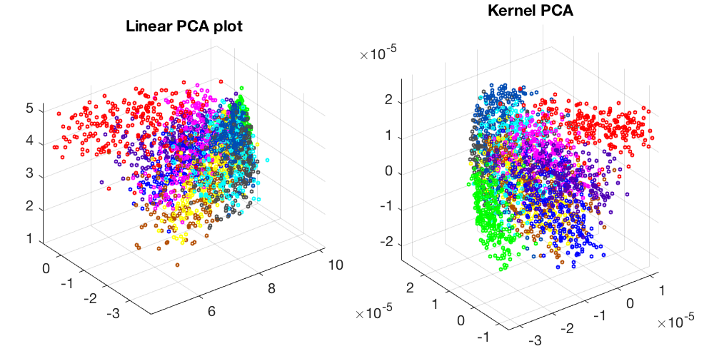
Visualization of a 256-D dataset of 10 classes of hand-written digits:

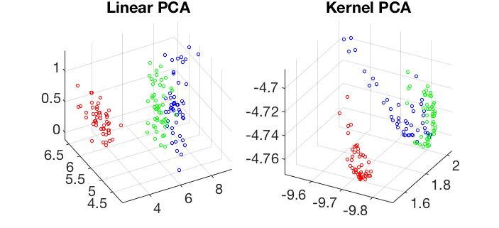
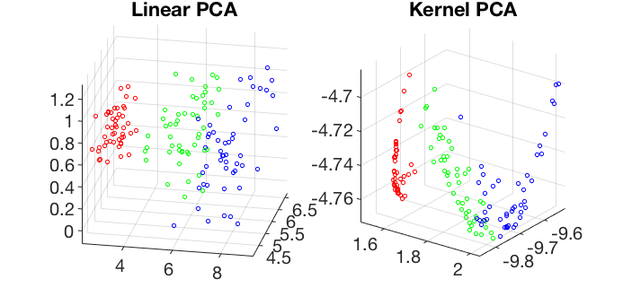
Visualization of the 4-D iris dataset in 3-D space spanned by the first 3 principal components of the linear and kernel PCA transforms: