Composite Rules

The Newton-Cotes quadrature rules estimate the integral of a function $f(x)$ over the integral interval $[a,\;b]$ based on an nth-degree interpolation polynomial as an approximation of $f(x)$, based on a set of $n+1$ points. To achieve higher accuracy, we need to increase the number of sample points $n$ to reduce the step size $h=(b-a)/n$, i.e., we need to use a higher degree polynomial to approximate $f(x)$. However, due to Runge's phenomenon, a high degree interpolation polynomial tends to result in oscillation at the edges of an interval and thereby causing large error.

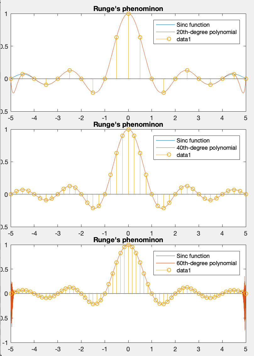
The figure below shows the approximation of the sinc function $f(x)=sin(x)/x$ by an nth-degree polynomials with $n=20,\,40,\,60$. Note that when $n=20$ is too low, the approximation is poor, but when $n=60$ is too high, Runge's phenonmenon is observed.

To avoid this problem, the composite quadrature rules can be used, which subdivides the entire integral interval $[a,\;b]$ into a set of $N$ subintervals each of size $h=(b-a)/N$ between every two consecutive sample points in $\{x_0,\cdots,x_N\}$, and estimates $I[f]$ as the sum of of the integrals over all such subintervals, each obtained by Newton-Cotes quadrature in Eq. (30) using a low-degree polynomial of degree $n$ based on $n+1$ subsample points in each subinterval (sharing the two end points with neighboring subintervals):

$$I[f]=\int_a^b f(x)dx=\sum_{j=0}^{N-1} \int_{x_j}^{x_{j+1}} f(x) dx \approx\sum_{j=0}^{N-1} \left(\sum_{i=0}^n c_{ij} f_{ij}\right)$$ (70)

where $f_{ij}$ is the ith function value in the jth subinterval weighted by the coefficient $c_{ij}$, which can be found as in Eq. (29) with $h$ replaced by $h/n=(b-a)/N/n$.

• Composite trapezoidal method ($n=1$):
  

  $$I[f] = \int_a^b f(x)dx=\sum_{j=0}^{N-1} \int_{x_j}^{x_{j+1}} f(x) dx \approx \;\sum_{j=0}^{N-1} \frac{h}{2}(f_j+f_{j+1})$$

  $$= \frac{h}{2}\left[f(a)+2\sum_{j=1}^{N-1}f_j+f(b)\right] =\frac{h}{2}[f(a)+f(b)]+h\,\sum_{j=1}^{N-1}f(a+jh)$$ (71)

  
  The error is:

  $$E_n[f]=-\sum_{j=0}^{N-1}\frac{h^3}{12}f''(\eta_j) =-\frac{h^3}{12}\sum_{j=0}^{N-1}f''(\eta_j), \;\;\;\;\;\;\eta_j\in(x_j,\,x_{j+1})$$ (72)

  But as

  $$\min_{0\le j\le n-1} f''(\eta_j) \le\frac{1}{n}\sum_{j=0}^{N-1}f''(\eta_j) \le \max_{0\le j\le n-1} f''(\eta_j)$$ (73)

  there must exist some $\eta\in(a,\,b)$ at which

  $$f''(\eta)=\frac{1}{n}\sum_{j=0}^{N-1} f''(\eta_j)$$ (74)

  $$E[f]=-\frac{h^3}{12}Nf''(\eta)=-\frac{(b-a)^3}{12\,N^2}f''(\eta)$$ (75)

  Obviously $E[f]$ is quickly reduced when $N$ is increased.

• Composite Simpson's rule ($n=2$):
  

  $$I[f] = \int_a^b f(x)\,dx=\sum_{j=0}^{N-1}\int_{x_j}^{x_{j+1}}f(x)\,dx \a... ...1}{2}\;\sum_{j=0}^{N-1}\frac{h}{3} \left[f(x_j)+4f(x_{j+1/2})+f(x_{j+1})\right]$$

  $$= \frac{h}{6}\left[f(a)+4\sum_{j=0}^{N-1}f(x_{j+1/2}) +2\sum_{j=1}^{N-1}f(x_j)+f(b)\right]$$

  $$= \frac{h}{6}\left[f(a)+4\sum_{j=0}^{N-1}f(a+(j+1/2)h) +2\sum_{j=1}^{N-1}f(a+jh)+f(b)\right]$$

  
  

  $$E_s[f]=-\frac{(h/2)^5}{90}\;N\,\sum_{j=0}^{N-1}f^{(4)}(\eta_j) =-... ...-a)^5}{90\,N^4} f^{(4)}(\eta) =-\frac{(b-a)^5}{2880}\frac{1}{n^4} f^{(4)}(\eta)$$ (76)

• Composite Simpson's 3/8 rule ($n=3$):
  

  $$I[f] = \int_a^b f(x)\,dx\approx \frac{1}{3}\sum_{j=0}^{N-1}\frac{3h}{8}\left[f(x_j)+3f(x_{j+1/3}) +3f(x_{j+2/3})+f(x_{j+1})\right]$$

  $$= \frac{h}{8}\left[f(a)+3\sum_{j=0}^{N-1}f(x_j+h/3) +3\sum_{j=0}^{N-1}f(x_j+2h/3)+2\sum_{j=1}^{N-1}f(x_j)+f(b)\right]$$

  
  

• Composite Boole's rule ($n=4$):
  

  $$I[f] = \int_a^b f(x)\,dx\approx \frac{1}{4}\sum_{j=0}^{N-1}\frac{2h}{45}\left[7f(x_j)+32f(x_{j+1/4}) +12f(x_{j+2/4})+32f(x_{j+3/4})+7f(x_{j+1})\right]$$

  $$= \frac{h}{90}\left[f(a)+32\sum_{j=0}^{N-1}f(x_j+h/4) +12\sum_{j=0}... ...f(x_j+2h/4)+32\sum_{j=0}^{N-1}f(x_j+3h/4) +14\sum_{j=1}^{N-1}f(x_j)+f(b)\right]$$

  
  

The Matlab function below estimates the integral of a given function $f(x)$ in interval $[a,\;b]$ by composite quadrature of degree $n$:

function CompositeQuadrature(f,a,b,n,N)     
    h=(b-a)/N;              % length of each of the N subintervals
    for n=1:4               % for each of the n polynomials
        I=0;
        c=coefs(n);         % quadrature coefficients of the nth polynomial
        for i=0:N-1         % for each of N intervals
            j=a+i*h;        % starting point for the ith interval
            for m=0:n       % add each of the n terms
                I(n)=I(n)+c(m+1)*f(j+m*h/n);
            end
        end
        I=h*I/n;
        fprintf('n=%d\tI=%f\n',n,I);
    end
end

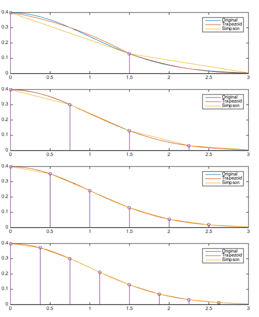
Example: Reconsider the integral in the previous example:

$$\int_0^3 g(x)\,dx=\frac{1}{\sqrt{2\pi}}\int_0^3 \exp\left(-\frac{x^2}{2}\right)\,dx$$ (77)

which is carried out by both the composite trapezoidal and Simpson's rules. The interval between $a=0$ and $b=3$ are divided into $N$ sub-intervals with $N=2,\;4,\;6$ and $8$. The results are listed in the table below. We see that in general the quadratic approximation by Simpson's method is of course more accurate than the linear approximation by the trapezoidal method. Also, when the interval $(a,\,b)$ is divided into more subintervals each approximated by either of the two methods, higher accuracy can be achieved.

$$\begin{tabular}{c\vert\vert c\vert l\vert l\vert l}\hline N & \mb... ...864956/5.45e-07 &0.4986499/2.43e-07&0.498650102/1.58e-10\\ \hline \end{tabular}$$

Taylor expansion of $f(x)$ around the middle point $x_{i+1/2}=(x_i+x_{i+1})/2$ between $x_i$ and $x_{i+1}$:

$$f(x)=f(x+h/2)+f'(x+h/2)\frac{h}{2}+\frac{f''(x+h/2)}{2}\left(\frac{h}{2}\right)^2+\cdots$$ (78)