Least square fitting

A generic data modeling problem can be formulated as the following: given a set of $N$ pairs of observed data points $\{(x_i, y_i),\; i=1,\cdots,N\}$, find a model $y=f(x,a_1,\cdots,a_M)$ to fit the relationship between the two variables $x$ and $y$:

$$y=f(x,a_1,\cdots,a_M)=f(x,{\bf a})$$ (17)

where ${\bf a}=[a_1,\cdots,a_M]^T$ is a set of $M$ parameters. We assume there are more data points than the number of parameters, i.e., $N>M$. In practice, $N$ is much greater than $M$. The error of the model for the ith data point is

$$e_i=y_i-f(x_i,{\bf a}),\;\;\;\;\;\;(i=1,\cdots,N)$$ (18)

Given the assumed function $y=f(x,a_1,\cdots,a_M)$, the goal is to find the $M$ optimal parameters for the model to best fit the data set, so that the following least squares (LS) error is minimized:

$$\varepsilon({\bf a})=\sum_{i=1}^Ne_i^2=\sum_{i=1}^N[y_i-f(x_i,{\bf a})]^2$$ (19)

If the $N$ data points $x_i$ can be assumed to be normally distributed random variables, then the LS-error is a random variable with chi-squared $\chi^2$-distribution of $N-M$ degrees of freedom.

For the LS-error $\varepsilon({\bf a})$ to be minimized, the optimal parameters $a_1,\cdots,a_M$ need to satisfy the following $M$ equations:

$$\frac{\partial}{\partial a_j}\varepsilon({\bf a}) = \frac{\partial}{\partial a_j}\sum_{i=1}^N \left[y_i-f(x_i,{\bf a}... ...2\sum_{i=1}^N [y_i-f(x_i,{\bf a})] \frac{\partial f(x_i,{\bf a})}{\partial a_j}$$

$$= -2\sum_{i=1}^N [y_i-f(x_i,{\bf a})] J_{ij}=0,\;\;\;\;\;(j=1,\cdots,M)$$ (20)

where $J_{ij}=\partial f(x_i,{\bf a})/\partial a_j$. We define ${\bf y}=[y_1,\cdots,y_N]^T$ and

$${\bf f}({\bf a})=\left[\begin{array}{c}f(x_1,{\bf a})\\ \vdots\\ f(x_N,{\bf a})\end{array}\right]_{N\times 1}$$ (21)

then the $N$ equations above can be written in vector form as the gradiant of $\varepsilon({\bf a})$:

$${\bf g}_\varepsilon({\bf a})=\frac{d}{d{\bf a}}\varepsilon({\bf a... ...rt\;\frac{d{\bf f({\bf a})}}{d{\bf a}} =-2{\bf J}^T\,({\bf y}-{\bf f}({\bf a}))$$ (22)

where ${\bf y}-{\bf f}({\bf a})$ is an N-D vector, and ${\bf J}$ is the $N\times M$ Jacobian matrix

$${\bf J}=\frac{d {\bf f}({\bf a})}{d{\bf a}} =\left[\begin{array}{... ...a_1 &\cdots& \partial f(x_N,{\bf a})/\partial a_M\end{array}\right]_{N\times M}$$ (23)

The optimal parameters can be obtained by solving a set of N nonlinear equations:

$${\bf J}^T\,({\bf y}-{\bf f}({\bf a}))={\bf0}$$ (24)

We first consider the special case of a linear model $y=f(x,a,b)=a+bx$, with the LS error:

$$\varepsilon=\sum_{i=1}^N[y_i-f(x_i,a,b)]^2 =\sum_{i=1}^N[y_i-(a+bx_i)]^2$$ (25)

The two parameters $a$ and $b$ can be found by solving these two equations:

$$\left\{ \begin{array}{l} \frac{\partial \varepsilon}{\partial a}=... ...on}{\partial b}=-2\left[\sum_{i=1}^N(y_i-a-bx_i)x_i\right]=0 \end{array}\right.$$ (26)

i.e.,

$$\left\{\begin{array}{l} Na+b\sum_{i=1}^N x_i=\sum_{i=1}^N y_i \\ a\sum_{i=1}^N x_i+b\sum_{i=1}^N x_i^2=\sum_{i=1}^N x_iy_i\end{array}\right.$$ (27)

Dividing both sides by $N$, we get

$$a=\bar{y}-b\bar{x},\;\;\;\;\; a\bar{x}+b\left(\frac{1}{N}\sum_{i=1}^N x_i^2\right) =\frac{1}{N}\sum_{i=1}^Nx_iy_i$$ (28)

where $\bar{x}$ and $\bar{y}$ are repectively the estimated means of $x$ and $y$:

$$\bar{x}=\frac{1}{N}\sum_{i=1}^Nx_i,\;\;\;\;\;\; \bar{y}=\frac{1}{N}\sum_{i=1}^Ny_i$$ (29)

Substituting the first equation $a=\bar{y}-b\bar{x}$ into the second, we get

$$(\bar{y}-b\bar{x})\bar{x}+b\;\frac{1}{N}\sum_{i=1}^Nx_i^2 =\frac{1}{N}\sum_{i=1}^Nx_iy_i$$ (30)

Solving for $b$ we get

$$b=\frac{\sum_{i=1}^Nx_iy_i/N-\bar{x}\bar{y}}{\sum_{i=1}^Nx_i^2/N-... ...y})/N}{\sum_{i=1}^N(x_i-\bar{x})^2/N} =\frac{\hat\sigma_{xy}^2}{\hat\sigma_x^2}$$ (31)

where $\hat\sigma_x^2$ and $\hat\sigma_{xy}^2$ are the estimated variance of $x$ and the estimated covariance of $x$ and $y$, respectively:

$$\hat\sigma_{xy}^2=\frac{1}{N}\sum_{i=1}^N(x_i-\bar{x})(y_i-\bar{y... ...\frac{1}{N}\sum_{i=1}^N(x_i-\bar{x})^2 =\frac{1}{N}\sum_{i=1}^N x_i^2-\bar{x}^2$$ (32)

Now we get

$$a=\bar{y}-\bar{x}\;\frac{\hat\sigma_{xy}^2}{\hat\sigma_x^2}$$ (33)

We next consider solving the least squares problems for nonlinear multi-variable models by the Gauss-Newton algorithm. Recall that to model the observed dataset $\{(x_i,\,y_i),\;(i=1,\cdots,N)\}$ by some model $y=f(x,{\bf a})$, we need to find the parameters in ${\bf a}$ that minimizes the squared error in Eq. (19), by solving the following equation (Eq. (24)):

$${\bf J}^T\,({\bf y}-{\bf f}({\bf a}))={\bf0}$$ (34)

This nonlinear equation system can be solved iteratively based on some initial guess ${\bf a}_0$:

$${\bf a}_{n+1}={\bf a}_n + \triangle {\bf a}_n,\;\;\;\;\;(n=0,1,2,\cdots)$$ (35)

To find the increment $\triangle {\bf a}_n={\bf a}_{n+1}-{\bf a}_n$ in the iteration, we consider the first two terms of the Taylor expansion of the function ${\bf f}({\bf a}_{n+1})$:

$${\bf f}({\bf a}_{n+1})={\bf f}({\bf a}_n+\triangle{\bf a}) \approx {\bf f}({\bf a}_n)+{\bf J}_n\triangle {\bf a} _n$$ (36)

where ${\bf J}_n$ is the $N\times M$ Jacobian matrix. Substituting this expression for $f({\bf a}_{n+1})$ into Eq. (34), we get

$${\bf J}^T_n({\bf y}-{\bf f}({\bf a}_{n+1})) \approx {\bf J}^T_n ({\bf y}-{\bf f}({\bf a}_n)-{\bf J}_n\triangle {\bf a}_n) ={\bf0}$$ (37)

i.e.,

$${\bf J}^T_n({\bf y}-{\bf f}({\bf a}_n)) ={\bf J}_n^T{\bf J}_n\triangle {\bf a}_n$$ (38)

Solving for $\triangle{\bf a}_n$ we get

$$\triangle {\bf a}_n=({\bf J}^T_n{\bf J}_n)^{-1}{\bf J}_n^T ({\bf y}-{\bf f}({\bf a}_n))={\bf J}_n^-({\bf y}-{\bf f}({\bf a}_n))$$ (39)

where ${\bf J}_n^-=({\bf J}^T_n{\bf J}_n)^{-1}{\bf J}_n^T$ is the pseudo inverse of ${\bf J}_n$. Now the iteration becomes:

$${\bf a}_{n+1}={\bf a}_n+\triangle{\bf a}_n ={\bf a}_n+{\bf J}_n^-({\bf y}-{\bf f}({\bf a}_n)) ={\bf a}_n-{\bf J}_n^-({\bf f}({\bf a}_n)-{\bf y})$$ (40)

Comparing this with the iteration used in Newton's method for solving a multivariate non-linear equation system ${\bf f}({\bf x})={\bf0}$:

$${\bf x}_{n+1}={\bf x}_n-{\bf J}_n^{-1}{\bf f}({\bf x}_n)$$ (41)

we see that the Gauss-Newton algorithm is essentially solving an over-constrained nonlinear equation system ${\bf f}({\bf a})-{\bf y}={\bf0}$. The optimal solution ${\bf a}^*$ will minimize $\vert\vert{\bf f}({\bf a})-{\bf y}\vert\vert$.

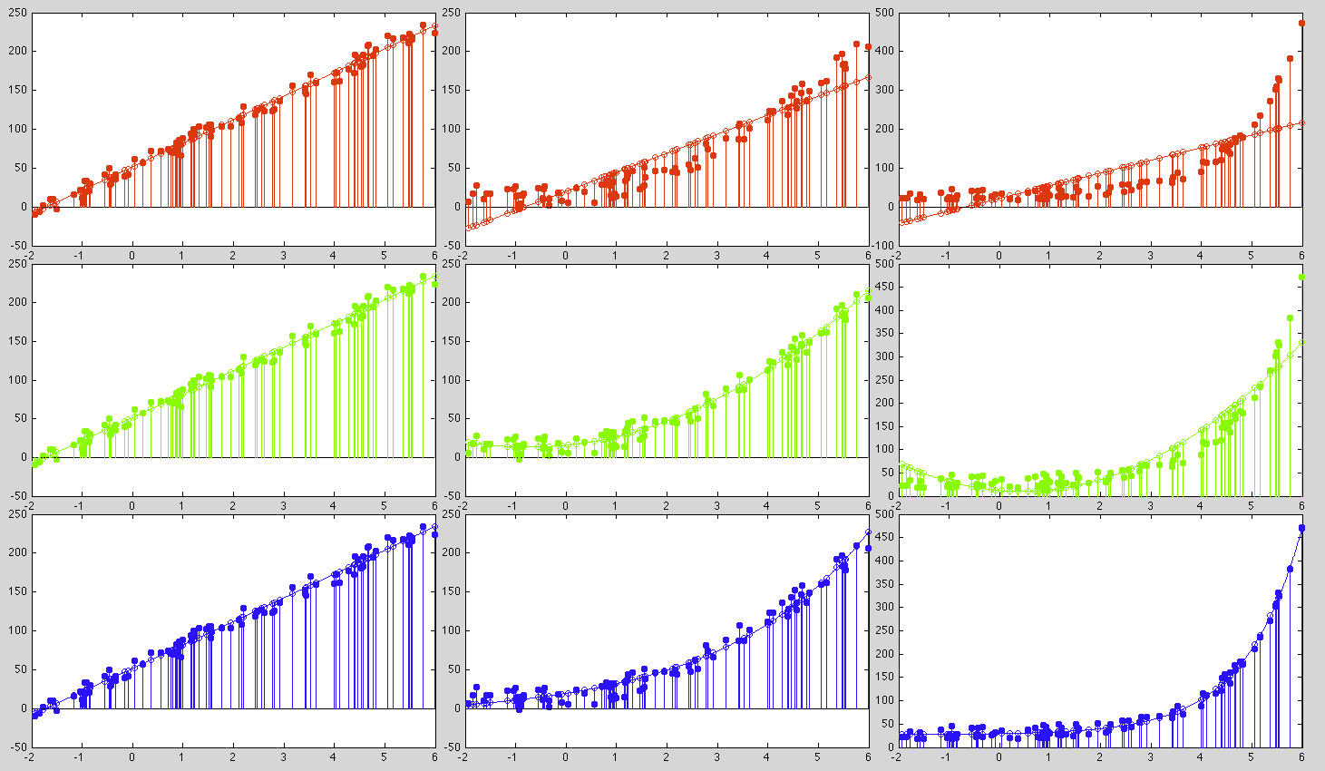
Example

Three sets of data (shown as the solid dots in the three columns in the plots below) are fitted by three different models (shown as the open circles in the plots):

1. Linear model:

   $$y=f_1(x)=ax+b$$ (42)

2. quadratic model:

   $$y=f_2(x)=ax^2+bx+c$$ (43)

3. Exponential model:

   $$y=f_3(x)=a\,e^{bx}+c$$ (44)

These are the parameters for the three models to fit each of the three data sets:

$$\begin{array}{r\vert\vert r\vert\vert r\vert r\vert r\vert\ve... ...del\;3: & 2.197 & 0.885 & 27.241 & 8.3393 \\ \hline \end{array}$$ (45)

We see that the first data set can be fitted by all three models equally well with similar error (when $a\approx 0$ in model 2, it is approximately a linear functions), the second dataset can be well fitted by either the second or the third model, while the third dataset can only be fitted by the third exponential model.