Interior Point Methods

Consider the a general constrained optimization problem:

$$\begin{tabular}{ll} min: & f({\bf x}) \\ s. t.: & $\left\{ \begi... ...{\bf g}({\bf x})\ge{\bf0}\\ {\bf x}\ge{\bf0} \end{array}\right.$ \end{tabular}$$ (237)

By introducing slack variables ${\bf s}\ge{\bf0}$, all inequality constraints can be converted into equality constraints:

$${\bf g}({\bf x})\le{\bf0}\;\Longrightarrow \; {\bf g}({\bf x})+{\... ...; {\bf g}({\bf x})\ge{\bf0}\;\Longrightarrow \; {\bf g}({\bf x})-{\bf s}={\bf0}$$ (238)

which can then be combined with the equality constraints and still denoted by ${\bf h}({\bf x})={\bf0}$, while the slack variables ${\bf s}$ are also combined with the original variables and still denoted by ${\bf x}$. We assume there are in total $M$ equality constraints and $N$ variables. Now the optimization problem can be reformulated as:

$$\begin{tabular}{ll} min: & f({\bf x}) \\ s. t.:& $\left\{\begin{... ...l} {\bf h}({\bf x})={\bf0}\\ {\bf x}\ge{\bf0} \end{array}\right.$\end{tabular}$$ (239)

The Lagrangian is

$$L({\bf x},{\bf\lambda},{\bf\mu})=f({\bf x}) +{\bf\lambda}^T{\bf h}({\bf x})-{\bf\mu}^T{\bf x}$$ (240)

The KKT conditions are

$$\left\{ \begin{array}{ll} \bigtriangledown_{\bf x} L({\bf x},... ... {\bf XM1}={\bf0} & \mbox{(complementarity)} \end{array}\right.$$ (241)

where ${\bf X}=diag(x_1,\cdots,x_N)$, ${\bf M}=diag(\mu_1,\cdots,\mu_N)$, and ${\bf J}_{\bf f}({\bf x})$ is the Jacobian matrix of ${\bf h}({\bf x})$:

$${\bf X}=\left[\begin{array}{ccc}x_1&\cdots&0\\ \vdots&\ddots&\vd... ...al x_1}&\cdots& \frac{\partial h_m}{\partial x_n}\end{array}\right]_{M\times N}$$ (242)

To simplify the problem, the non-negativity constraints can be removed by introducing an indicator function:

$$I(x)=\left\{\begin{array}{ll}0 & x\ge 0\\ \infty& x<0\end{array}\right.$$ (243)

which, when used as a cost function, penalizes any violation of the non-negativity constraint $x\ge 0$. Now the optimization problem can be reformulated as shown below without the non-negative constants ${\bf x}\ge{\bf0}$:

$$\begin{tabular}{ll} min: & $f({\bf x})+\sum_{i=1}^N I(x_i)$\ \\ s. t.: & ${\bf h}({\bf x})={\bf0}$ \end{tabular}$$ (244)

However, as the indicator function is not smooth and therefore not differentiable, it is approximated by the logarithmic barrier function which approaches $I(x)$ when the parameter $t>0$ approaches infinity:

$$-\frac{1}{t}\ln(x)\;\;\stackrel{t\rightarrow\infty}{\Longrightarrow}\;\;I(x)$$ (245)

Now the optimization problem can be written as:

$$\begin{tabular}{ll} min: & $f({\bf x})-\frac{1}{t}\sum_{i=1}^N\ln x_i$\ \\ s. t.: & ${\bf h}({\bf x})={\bf0}$ \end{tabular}$$ (246)

The Lagrangian is:

$$L({\bf x},{\bf\lambda},{\bf\mu})=f({\bf x}) +{\bf\lambda}^T{\bf h}({\bf x})-\frac{1}{t}\sum_{j=1}^N\ln x_j\\$$ (247)

and its gradient is:

$$\bigtriangledown_{\bf x} L({\bf x},{\bf\lambda},{\bf\mu}) ={\bf g... ...{\bf x})+{\bf J}_{\bf h}^T({\bf x}){\bf\lambda} -\frac{1}{t}{\bf X}^{-1}{\bf 1}$$ (248)

We define

$${\bf\mu}=\frac{\bf x}{t}=\frac{1}{t}{\bf X}^{-1}{\bf 1}, \;\;\;\; \;\;\; {\bf X\mu}={\bf XM 1}=\frac{\bf 1}{t}$$ (249)

and combine this equation with the KKT conditions of the new optimization problem to get

$$\left\{ \begin{array}{ll} {\bf g}_f({\bf x})+{\bf J}_{\bf h}^... ...-{\bf 1}/t={\bf0} & \mbox{(complementarity)} \end{array}\right.$$ (250)

The third condition is actually from the definition of ${\bf\mu}$ given above, but here it is labeled as complementarity, so that these conditions can be compared with the KKT conditions of the original problem. We see that the two sets of KKT conditions are similar to each other, with the following differences:

• The non-negativity ${\bf x}\ge{\bf0}$ in the primal feasibility of the original KKT is dropped;
• Consequently the inequality ${\bf\mu}\ge{\bf0}$ in the dual feasibility of the original KKT conditions is also dropped;
• There is an extra term ${\bf 1}/t$ in complementarity which will vanish when $t\rightarrow\infty$.

The optimal solution that minimizes the objective function $f({\bf x})$ can be found by solving the simultaneous equations in the modified KKT conditions (with no inequalities) given above. To do so, we first express the equations in the KKT conditions above as a nonlinear equation system ${\bf F}({\bf x},{\bf\lambda},{\bf\mu})={\bf0}$, and find its Jacobian matrix ${\bf J}_{\bf F}$ composed of the partial derivatives of the function ${\bf F}({\bf x},{\bf\lambda},{\bf\mu})$ with respect to each of the three variables ${\bf x}$, ${\bf\lambda}$, and ${\bf\mu}$:

$${\bf F}({\bf x},{\bf\lambda},{\bf\mu})=\left[ \begin{array}{c} {\... ... h}({\bf x}) & {\bf0} & {\bf0} \\ {\bf M} & {\bf0} & {\bf X}\end{array}\right]$$ (251)

where

$${\bf W}({\bf x}) = \bigtriangledown_{\bf x} \left[{\bf g}_f({\bf x})+{\bf J}_{\bf h}^T({\bf x}){\bf\lambda} -{\bf\mu}\right]$$

$$= \bigtriangledown_{\bf x} {\bf g}_f({\bf x}) -\bigtriangledown_{\b... ...l x_N}\right]^T ={\bf H}_f({\bf x})-\sum_{i=1}^M\lambda_i{\bf H}_{h_i}({\bf x})$$ (252)

is symmetric as the Hessian matrices ${\bf H}_f$ and ${\bf H}_{h_i},\; (i=1,\cdots,M)$ are symmetric.

We can now use the Newton-Raphson method to find the solution of the nonlinear equation ${\bf F}({\bf x},{\bf\lambda},{\bf\mu})={\bf0}$ iteratively:

$$\left[\begin{array}{c}{\bf x}_{n+1}\\ {\bf\lambda}_{n+1}\\ {\bf\... ...{c}\delta{\bf x}_n\\ \delta{\bf\lambda}_n\\ \delta{\bf\mu}_n\end{array}\right]$$ (253)

where $\alpha$ is a parameter that controls the step size and $[\delta{\bf x}_n,\delta{\bf\lambda}_n,\delta{\bf\mu}_n]^T$ is the search direction (Newton direction), which can be found by solving the following equation:

$${\bf J}_{\bf F}({\bf x}_n,{\bf\lambda}_n,{\bf\mu}_n) \left[\begin... ...c} \delta{\bf x}_n\\ \delta{\bf\lambda}_n\\ \delta{\bf\mu}_n \end{array}\right]$$

$$= -{\bf F}({\bf x}_n,{\bf\lambda}_n,{\bf\mu}_n) =-\left[\begin{arra... ...bda}_n-\mu_n\\ {\bf h}({\bf x}_n)\\ {\bf X_nM_n1}-{\bf 1}/t \end{array}\right]$$ (254)

To get the initial values for the iteration, we first find any point inside the feasible region ${\bf x}_0$ and then ${\bf\mu}_0={\bf x}_0/t$, based on which we further find ${\bf\lambda}_0$ by solving the first equation in the KKT conditions in Eq. (250).

Actually this equation system above can be separated into two subsystems, which are easier to solve. Pre-multiplying ${\bf X}^{-1}$ to the third equation:

$${\bf M}\delta{\bf x}+{\bf X}\delta{\bf\mu}=-{\bf XM1}+{\bf 1}/t$$ (255)

we get

$${\bf X}^{-1}{\bf M}\delta{\bf x}+\delta{\bf\mu} =-{\bf M1}+{\bf X}^{-1}{\bf 1}/t=-{\bf\mu}+{\bf X}^{-1}{\bf 1}/t$$ (256)

Adding this to the first equation:

$${\bf W}\delta{\bf x}+ {\bf J}^T_{\bf h}({\bf x}) \delta{\bf\lambd... ...lta{\bf\mu}=-{\bf g}_f({\bf x})-{\bf J}_{\bf h}^T({\bf x}){\bf\lambda}+{\bf\mu}$$ (257)

we get

$$({\bf W}+{\bf X}^{-1}{\bf M})\delta{\bf x}+{\bf J}^T_{\bf h}({\bf... ...\bf X}^{-1}{\bf 1}/t =-\bigtriangledown_{\bf x}L({\bf x},{\bf\lambda},{\bf\mu})$$ (258)

Combining this equation with the second one, we get an equation system of two vector variables $\delta{\bf x}$ and $\delta{\bf\lambda}$ with symmetric coefficient matrix:

$$\left[\begin{array}{ccc} {\bf W}+{\bf X}^{-1}{\bf M} & {\bf J}^T_... ..._{\bf x}L({\bf x},{\bf\lambda},{\bf\mu})\\ {\bf h}({\bf x}) \end{array}\right]$$ (259)

Solving this equation system we get $\delta{\bf x}$ and $\delta{\bf\lambda}$, and we can further find $\delta{\bf\mu}$ by solving the third equation

$${\bf M}\delta{\bf x}+{\bf X}\delta\mu=-{\bf XM1}-{\bf 1}/t$$ (260)

to get

$$\delta{\bf\mu}={\bf X}^{-1}{\bf 1}/t-{\bf X}^{-1}{\bf M}\delta{\bf x}-{\bf\mu}$$ (261)

We now consider the two special cases of linear and quadratic programming:

• Linear programming:

  $$\begin{tabular}{ll} min: & $f({\bf x})={\bf c}^T{\bf x}$\ \\ s. ... ...bf h}({\bf x})={\bf Ax}-{\bf b}={\bf0}, \;\;\;\;{\bf x}\ge{\bf0}$ \end{tabular}$$ (262)

  We have
  • ${\bf g}_f({\bf x})=\bigtriangledown_{\bf x}f({\bf x})={\bf c}$
  • ${\bf J}_{\bf h}({\bf x})=\bigtriangledown_{\bf x}({\bf Ax}-{\bf b})={\bf A}$.
  • ${\bf W}({\bf x})=\bigtriangledown^2_{\bf x} L({\bf x},{\bf\lambda},{\bf\mu})={\bf0}$.
  The Lagrangian is

  $$L({\bf x},{\bf\lambda},{\bf\mu}) ={\bf c}^T{\bf x}+{\bf\lambda}^T({\bf Ax}-{\bf b})-{\bf\mu}^T{\bf x}$$ (263)

  The KKT conditions are:

  $$\left\{ \begin{array}{ll} \bigtriangledown_{\bf x} L({\bf x},... ...bf0} \nonumber\\ {\bf XM1}-{\bf 1}/t={\bf0} \end{array}\right.$$

  The search direction of the iteration can be found by solving the this equation system:

  $$\left[\begin{array}{ccc} {\bf0} & {\bf A}^T & -{\bf I}\\ {\bf A}... ...f\lambda}-{\bf\mu}\\ {\bf Ax}-{\bf b}\\ {\bf XM1}-{\bf 1}/t \end{array}\right]$$ (264)

  By solving the equation ${\bf c}+{\bf A}^T{\bf\lambda}-{\bf\mu}={\bf0}$ we get the initial value ${\bf\lambda}$. The Matlab code for the interior point method for the LP problem is listed below:

  function x=InterierPointLP(A,c,b,x)
      % given A,b,c of the LP problem and inital value of x,
      % find optimal solution x that minimizes c'*x
      [m n]=size(A);      % m constraints, n variables
      z1=zeros(n);
      z2=zeros(m);        % zero matrices in coefficient matrix
      z3=zeros(m,n);
      I=eye(n);           % identity matrix in coefficient matrix
      y=ones(n,1);
      t=9;                % initinal value for parameter t
      alpha=0.3;          % small enough not to exceed boundary
      mu=x./t;
      lambda=pinv(A')*(mu-c); % initial value of lambda
      w=[x; lambda; mu];      % initial values for all three 
      B=[c+A'*lambda-mu; A*x-b; x.*mu-y/t];   
      p=[x(1) x(2)];      % initial guess of solution
      while norm(B)>10^(-7)        
          t=t*9;          % increase parameter t
          X=diag(x);
          M=diag(mu);
          C=[z1 A' -I; A z2 z3; M z3' X];
          B=[c+A'*lambda-mu; A*x-b; x.*mu-y/t]; 
          dw=-inv(C)*B;  	% find search direction
          w=w+alpha*dw;   % step forward
          x=w(1:n);
          lambda=w(n+1:n+m);
          mu=w(n+m+1:length(w));       
          p=[p; x(1), x(2)];
      end
      scatter(p(:,1),p(:,2));  % plot trajectory of solution
  end
  

  Example:

  A given linear programming problem shown below is first converted into the standard form:

  $$\begin{tabular}{ll} max: & $f(x_1,x_2)=2x_1+3x_2$\ \\ s. t.: & $... ...1+5x_2+x_5=40 \\ x_i \ge 0,\;\;(i=1,\cdots,5) \end{array}\right.$ \end{tabular}$$

  or in matrix form:

  $$\begin{tabular}{ll} min: & $f({\bf x})={\bf c}^T{\bf x}$\ \\ s. ... ... h}({\bf x})={\bf A}{\bf x}-{\bf b}={\bf0},\;\;{\bf x}\ge {\bf0}$ \end{tabular}$$

  with

  $${\bf x}=\left[\begin{array}{c}x_1\\ x_2\\ x_3\\ x_4\\ x_5\end{arr... ...y}\right],\;\;\;\; {\bf b}=\left[\begin{array}{c}18\\ 60\\ 40\end{array}\right]$$

  where $x_3,\,x_4,\,x_5$ are the slack variables.

  

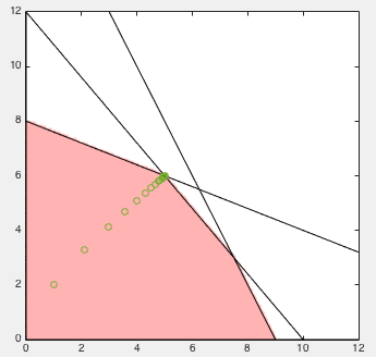
  We choose an initial value ${\bf x}_0=[1,\,2,\,1,\,1,\,1]^T$, and an initial parameter $t=9$, which is scaled up by a factor of $9$ in each iteration. We also used full Newton step size of $\alpha=1$. After 8 iterations, the algorithm converged to the optimal solution ${\bf x}^*=[5,\;6]^T$ corresponding to the maximum function value $f({\bf x}^*)=2x_1+3x_2=28$:

  $$\begin{array}{c\vert\vert c c\vert c \vert c}\hline & (x_1 & ... ...0 & 6.000000e+00) & -28.000000 & 0.000000 \\ \hline \end{array}$$

  At the end of the iteration, we also get the values of the slack variables: $x_3=2,\;x_4=x_5=0$.

• Quadratic programming:

  $$\begin{tabular}{ll} min: & $f({\bf x})=\frac{1}{2}{\bf x}^T{\bf Q... ...{\bf x})={\bf A}{\bf x}-{\bf b}={\bf0}, \;\;\;\;{\bf x}\ge{\bf0}$ \end{tabular}$$ (265)

  We have
  • ${\bf g}_f({\bf x})=\bigtriangledown_{\bf x}f({\bf x})={\bf Qx}+{\bf c}$
  • ${\bf J}_{\bf h}({\bf x})=\bigtriangledown_{\bf x}({\bf Ax}-{\bf b})={\bf A}$.
  • ${\bf W}({\bf x})=\bigtriangledown^2_{\bf x} L({\bf x},{\bf\lambda},{\bf\mu})={\bf Q}$.
  The Lagrangian is

  $$L({\bf x},{\bf\lambda},{\bf\mu}) =\frac{1}{2}{\bf x}^T{\bf Qx}+{\bf c}^T{\bf x} +{\bf\lambda}^T({\bf Ax}-{\bf b})-{\bf\mu}^T{\bf x}$$ (266)

  The KKT conditions are:

  $$\left\{ \begin{array}{ll} \bigtriangledown_{\bf x} L({\bf x},... ...bf0} \nonumber\\ {\bf XM1}-{\bf 1}/t={\bf0} \end{array}\right.$$

  The equation system for the Newton-Raphson method is:

  $$\left[\begin{array}{ccc} {\bf Q} & {\bf A}^T & -{\bf I}\\ {\bf A... ...f\lambda}-{\bf\mu}\\ {\bf Ax}-{\bf b}\\ {\bf XM1}-{\bf 1}/t \end{array}\right]$$ (267)

The Matlab code for the interior point method for the QP problem is listed below:

function [x mu lambda]=InteriorPointQP(Q,A,c,b,x)
    n=length(c);        % n variables
    m=length(b);    	% m constraints
    z2=zeros(m);
    z3=zeros(m,n);
    I=eye(n);
    y=ones(n,1);
    t=9;                % initinal value for parameter t
    alpha=0.1;       	% stepsize, small enough not to exceed boundary
    mu=x./t;
    lambda=pinv(A')*(mu-c-Q*x); % initial value of lambda
    w=[x; lambda; mu];   	% initial value
    B=[Q*x+c+A'*lambda-mu; A*x-b; x.*mu-y/t];             
    while norm(B)>10^(-7)   
        t=t*9;        	% increase parameter t
        X=diag(x);
        M=diag(mu);       
        C=[Q A' -I; A z2 z3; M z3' X];
        B=[Q*x+c+A'*lambda-mu; A*x-b; x.*mu-y/t];             
        dw=-inv(C)*B;  	% find search direction
        w=w+alpha*dw;  	% step forward
        x=w(1:n);
        lambda=w(n+1:n+m);
        mu=w(n+m+1:length(w));
    end
end

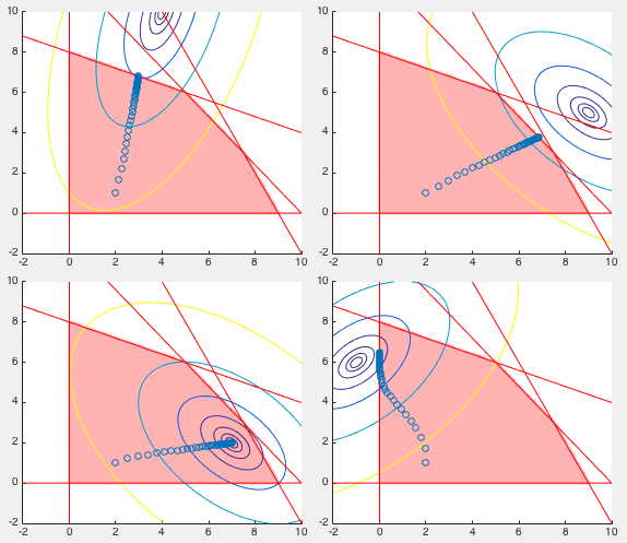
Example:

A 2-D quadratic programming problem shown below is to minimize four different quadratic functions under the same linear constraints as the liniear programming problem in the previous example. In general, the quadratic function is given in the matrix form:

$$\begin{tabular}{ll} min: & $f({\bf x})=[{\bf x}-{\bf m}]^T{\bf Q}... ... h}({\bf x})={\bf A}{\bf x}-{\bf b}={\bf0},\;\;{\bf x}\ge {\bf0}$ \end{tabular}$$

with following four different sets of function parameters:

$${\bf Q}=\left[\begin{array}{rr}4 & -1\\ -1 & 4\end{array}\right],... ...d{array}\right],\;\;\; \left[\begin{array}{rr}3 & -1\\ -1 & 3\end{array}\right]$$

$${\bf m}=\left[\begin{array}{r}4\\ 10\end{array}\right],\;\;\; \le... ...r}7\\ 2\end{array}\right],\;\;\; \left[\begin{array}{r}-1\\ 6\end{array}\right]$$

As shown in the four panels in the figure below, the iteration of the interior point algorithm brings the solution from the same initial position at ${\bf x}_0=[2,\;1]^T$ to the final position for each of the four objective functions $f({\bf x})$, the optimal solution, which is on the boundary of the feasible region in all cases except the third one, where the optimal solution is inside the feasible region, i.e., the optimization problem is not constrained. Also note that the trajectories of the solution during the iteration go straightly from the initial guess to the final optimal solution by following the negative gradient direction of the quadratic function in all cases execpt in the last one, where it makes a turn while approaching the vertical boundary, due obviously to the significantly greater value of the log barrier function close to the boundary.