Next: The Simplex Algorithm Up: Constrained Optimization Previous: Duality and KKT Conditions
The basic problem in linear programming (LP) is to minimize/maximize a
linear objective function
 of
of  variables
 under a set of
  linear constraints:
 |
(209) |
The LP problem can be more concisely represented in matrix form:
where![$\displaystyle {\bf x}=\left[\begin{array}{c}x_1\\ \vdots\\ x_N\end{array}\right...
...ts&a_{1N}\\
\vdots & \ddots & \vdots \\ a_{M1}&\cdots&a_{MN}\end{array}\right]$](img789.svg) |
(211) |
For example, the objective function could be the total profit,
the constraints could be some limited resources. Spicifically,
may represent the quantities of different
types of products,
 represent their unit prices,
and
represent their unit prices,
and  represent the consumption of the ith resource by
the jth product, the goal is to maximize the profit
represent the consumption of the ith resource by
the jth product, the goal is to maximize the profit
 subject to the constraints imposed by
the limited resources
subject to the constraints imposed by
the limited resources
 .
.
Here all variables are assumed to be non-negative. If there exists a variable that is not restricted, it can be eliminated. Specifically, we can solve one of the constraining equations for the variable and use the resulting expression of the variable to replace all its appearances in the problem. For example:
 |
(212) |
 , we get
 . Substituting this into the objective
function and the other constraint, we get
. Substituting this into the objective
function and the other constraint, we get
 and
and
 , the problem can be reformulated as:
 |
(213) |
Given the primal LP problem above, we can further find its dual problem. We first construct the Lagrangian of primal problem:
 |
(214) |
![${\bf y}=[y_1,\cdots,y_M]^T$](img800.svg) contains the Lagrange multipliers
for the inequality constraints
contains the Lagrange multipliers
for the inequality constraints
 , and
, and
 according to Table 188. We
define the dual function as the maximum of
according to Table 188. We
define the dual function as the maximum of
 over
over
 :
:
![$\displaystyle f_d({\bf y})=\max_{\bf x} L({\bf x})
=\max_{\bf x} [ {\bf c}^T{\b...
...bf b}) ]
=\max_{\bf x} [ ({\bf c}-{\bf A}^T{\bf y})^T{\bf x}+{\bf y}^T{\bf b} ]$](img804.svg) |
(215) |
that maximizes
, we set
its gradient to zero and get:
![$\displaystyle \bigtriangledown_{\bf x}L({\bf x})
=\bigtriangledown_{\bf x}[ ({\...
...}-{\bf A}^T{\bf y})^T{\bf x}+{\bf y}^T{\bf b}]
={\bf c}-{\bf A}^T{\bf y}={\bf0}$](img805.svg) |
(216) |
 we get:
 , which is the upper bound of
 , under the constraint that
 so that
 contributes negatively
to
(as
contributes negatively
to
(as
 ):
):
 |
(217) |
 ,
to become the tightest upper bound, i.e., the original primal
problem of maximization in Eq. (210) has now been converted
into the following dual problem of minimization:
,
to become the tightest upper bound, i.e., the original primal
problem of maximization in Eq. (210) has now been converted
into the following dual problem of minimization:
 |
(218) |
 |
(219) |
If either the primal or the dual is feasible and bounded, so is
the other, and they form a strong duality, the solution  of
the dual problem is the same as the solution
of
the dual problem is the same as the solution  of the primal
problem. Also, as the primal and dual problems are completely
symmetric.
of the primal
problem. Also, as the primal and dual problems are completely
symmetric.
An inequality constrained LP problem can be converted to an equality constrained problem by introducing slack variables:
 |
(220) |
 |
(221) |
is an  dimensional augmented variable vector that
includes the slack variables
dimensional augmented variable vector that
includes the slack variables
 as well as the
original variables
as well as the
original variables
 :
:
![$\displaystyle {\bf x}=[x_1,\;x_2,\cdots,x_N,\,s_1,\;s_2,\cdots,s_M]^T$](img823.svg) |
(222) |
 is redefined as an
 augmented coefficient
matrix that includes coefficients for both types of variables:
augmented coefficient
matrix that includes coefficients for both types of variables:
![$\displaystyle {\bf A}=\left[\begin{array}{cccc\vert cccc}
a_{11} & a_{12} & \cd...
...\right]_{M\times (N+M)}
=[\;{\bf A}_{M\times N}\;\vert\; {\bf I}_{M\times M}\;]$](img825.svg) |
(223) |
 are the coefficients for the
original variables
, and the identity matrix
are the coefficients for the
original variables
, and the identity matrix
![${\bf I}_{M\times M}=[{\bf e}_1,\cdots,{\bf e}_M]$](img827.svg) is for the unity
coefficients of the slack variables
,
each of which appears in the constraints only once.
is for the unity
coefficients of the slack variables
,
each of which appears in the constraints only once.
Now the LP problem can be expressed in the standard form (original form
on the left, with and redefined on the right):
 or or |
(224) |
An LP problem can be viewed geometrically. If normalize
 so that
 , then the objective function
 becomes the projection of
onto . Each of the equality constraints in
becomes the projection of
onto . Each of the equality constraints in
 represents a hyper-plane in the N-D
vector space perpendicular to its normal direction
represents a hyper-plane in the N-D
vector space perpendicular to its normal direction
![${\bf a}_j=[a_{i1},\cdots,a_{IN}]^T$](img833.svg) :
:
 |
(225) |
non-negativity conditions  in
in
 corresponds to a hyper-plane perpendicular
to the jth standard basis vector
corresponds to a hyper-plane perpendicular
to the jth standard basis vector  . In general, in an
N-D space, if none of the hyper-planes is parallel to any others,
then no more than hyper-planes intersect at one point. For
example, in a 2-D or 3-D space, two straignt lines or three
surfaces intersect at a point. Here for the LP problem in the
N-D space, the total number of intersection points formed by
the hyper-planes is
. In general, in an
N-D space, if none of the hyper-planes is parallel to any others,
then no more than hyper-planes intersect at one point. For
example, in a 2-D or 3-D space, two straignt lines or three
surfaces intersect at a point. Here for the LP problem in the
N-D space, the total number of intersection points formed by
the hyper-planes is
 |
(226) |
The polytope enclosed by these hyper-planes is called the
feasible region, in which the optimal solution must lie. The
vertices of the polytopic feasible region are a subset
of the  intersections.
Fundamental theorem of linear programming
The optimal solution  of a linear programming problem
formulated above is either a vertex of the polytopic feasible
region
of a linear programming problem
formulated above is either a vertex of the polytopic feasible
region  , or lies on a hyper-surface of the polytope, on which
all points are optimal solutions.
, or lies on a hyper-surface of the polytope, on which
all points are optimal solutions.
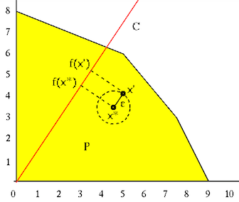
Proof:
Assume the optimal solution
 is interior to
the polytopic feasible region , then there must exist some
is interior to
the polytopic feasible region , then there must exist some
 such that the hyper-sphere of radius
  centered at is inside . Evaluate the objective
function at a point on the hyper-sphere
centered at is inside . Evaluate the objective
function at a point on the hyper-sphere
 |
(227) |
 |
(228) |
cannot be the optimal solution as assumed. This contradiction
indicates that an optimal solution must be on the surface of ,
either at one of its vertices or on one of its surfaces. Q.E.D.
Based on this theorem, the optimization of a linear programming problem
could be solved by exhaustively checking each of the  intersections
formed by of the hyper-planes to find (a) whether it is feasible
(satisfying all constraints), and, if so, (b) whether the objective
function
intersections
formed by of the hyper-planes to find (a) whether it is feasible
(satisfying all constraints), and, if so, (b) whether the objective
function
 is maximized at the point. Specifically, we choose
of the equations for the the constraints and solve this N-equation
and N-unknown linear system to get the intersection point of corresponding
hyper-planes. This brute-force method is most straight forward, but the
computational complexity is high when and , and therefore ,
become large.
is maximized at the point. Specifically, we choose
of the equations for the the constraints and solve this N-equation
and N-unknown linear system to get the intersection point of corresponding
hyper-planes. This brute-force method is most straight forward, but the
computational complexity is high when and , and therefore ,
become large.
Example:
 or or |
![$\displaystyle {\bf x}=\left[\begin{array}{c}x_1\\ x_2\end{array}\right],\;\;\;\...
...ight],\;\;\;\;
{\bf A}=\left[\begin{array}{cc}2&1\\ 6&5\\ 2&5\end{array}\right]$](img847.svg) |
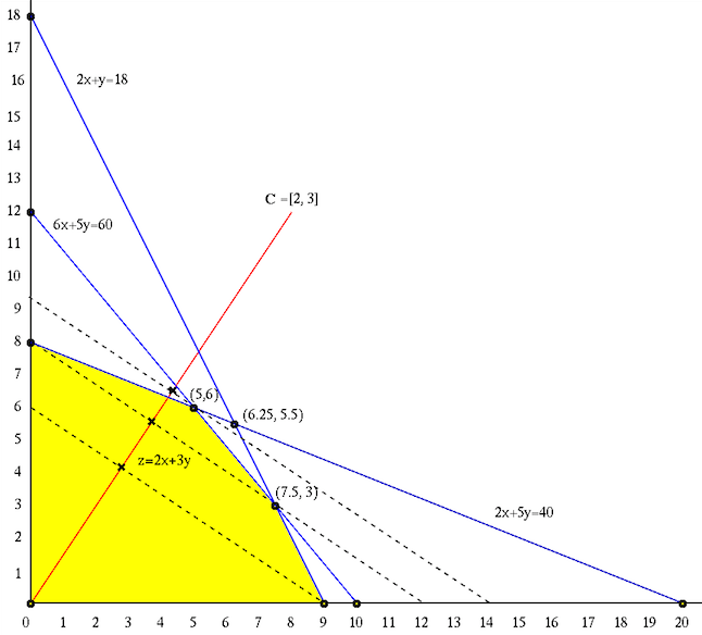
This problem has  variables with the same number of non-negativity
constraints and
variables with the same number of non-negativity
constraints and  linear inequality constraints. The
  straight
lines form
straight
lines form
 intersections, out of which 5 are the
vertices of the polygonal feasible region satisfying all constraints.
The value of the objective function
intersections, out of which 5 are the
vertices of the polygonal feasible region satisfying all constraints.
The value of the objective function
 is proportional to the projection of the 2-D variable vector
![${\bf x}=[x_1,\;x_2]^T$](img852.svg) onto the coefficient vector
onto the coefficient vector
![${\bf c}=[2,\;3]^T$](img853.svg) .
The goal of this linear programming problem is to find a point
inside the polygonal feasible region with maximum
(the projection of onto
vector if
). Geometrically, this can be
understood as to push the hyper-plane
.
The goal of this linear programming problem is to find a point
inside the polygonal feasible region with maximum
(the projection of onto
vector if
). Geometrically, this can be
understood as to push the hyper-plane
 , here a
line in 2-D space, its normal direction , away from the
origin along to eventually arrive at the vertex of the polytopic
feasible region farthest away from the origin.
, here a
line in 2-D space, its normal direction , away from the
origin along to eventually arrive at the vertex of the polytopic
feasible region farthest away from the origin.
This LP problem can be converted into the standard form:
 |
Listed in the table below are the
 intersections
, called basic solutions, together with the corresponding
slack variables
intersections
, called basic solutions, together with the corresponding
slack variables
 and the objective function value
(proportional to the projection of onto
). We see that out of the ten basic solutions, five are
feasible (vertices of the polytopic feasible region) with all
and the objective function value
(proportional to the projection of onto
). We see that out of the ten basic solutions, five are
feasible (vertices of the polytopic feasible region) with all
 variables taking non-negative values, while the remaining
five are not feasible, as some of the slack variables are negative,
and thereby violating the constraints. Out of the five feasible
solutions, the one at
variables taking non-negative values, while the remaining
five are not feasible, as some of the slack variables are negative,
and thereby violating the constraints. Out of the five feasible
solutions, the one at
 is optimal with maximum
objective function value
is optimal with maximum
objective function value
 .
.
 |
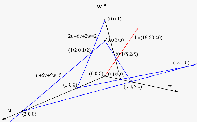
This primal maximization problem can be converted into the dual minimization problem:
 or or |
The five planes,  from the constraining inequalities, and
  for the non-negative constraints
  ,
,  , and
, and  for the three variables, form
  intersection points:
 |
We see that at the feasible point
 , the dual function
 is minimized to be
  , the same
as the maximum of the primal function
, the same
as the maximum of the primal function
 at
at  .
.
Homework:
Develop the code to find all intersections formed by
given hyper-planes in an N-D space in terms of their
equations
 and
, identify which of them are vertices of
the polytope surrounded by these hype-planes, and find the vertex
corresponding to the optimal solution that maximizes
for a given .
and
, identify which of them are vertices of
the polytope surrounded by these hype-planes, and find the vertex
corresponding to the optimal solution that maximizes
for a given .
