Next: Duality and KKT Conditions Up: Constrained Optimization Previous: Optimization with Equality Constraints
The optimization problems subject to inequality constraints can be generally formulated as:
 |
(185) |
 and
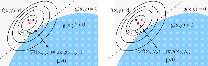
and  , as shown in the figure below for the minimization
(left) and maximization (right) of
, as shown in the figure below for the minimization
(left) and maximization (right) of
 subject to
 . The constrained solution
![${\bf x}^*=[x^*_1,\,x^*_2]^T$](img691.svg) is on the boundary of the feasible region satisfying
is on the boundary of the feasible region satisfying
 ,
while the unconstrained extremum is outside the feasible region.
,
while the unconstrained extremum is outside the feasible region.
Consider the following two possible cases.
 is outside the feasible
region, i.e., the inequality constraint is active, then the
constrained solution
is outside the feasible
region, i.e., the inequality constraint is active, then the
constrained solution  must be
 ,
,
 ;
and the constraining function
;
and the constraining function
 to have the same tangent
at , or parallel gradients:
to have the same tangent
at , or parallel gradients:
 or or |
(186) |
 or
or  , respectively, as illustrated in the 1-D examples in
the figure below:
, respectively, as illustrated in the 1-D examples in
the figure below:
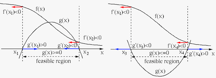
Depending on whether
is to be maximized or minimized,
and whether the constraint is
 or
or
 ,
there exist four possible cases in terms of the sign of
,
there exist four possible cases in terms of the sign of  , as
summarized in the table below:
, as
summarized in the table below:
 |
(187) |
and
for either maximization or minimization:
of this unconstrained
problem is
 ;
;
 ;
;
 and find the solution solving the
same equation
and find the solution solving the
same equation

Summarizing the two cases above, we see that
but
 in the first case,
but
in the first case,
but  in the second case, i.e., the following holds in either case:
The discussion above can be generalized from 2-D to  dimensional
space, in which the optimal solution is to be found
to extremize the objective
subject to
dimensional
space, in which the optimal solution is to be found
to extremize the objective
subject to  inequality
constraints
inequality
constraints
 . To solve this inequality
constrained optimization problem, we first construct the Lagrangian:
. To solve this inequality
constrained optimization problem, we first construct the Lagrangian:
 |
(191) |
indicated in Table 188
is negated.
We now set the gradient of the Lagrangian to zero:
![$\displaystyle \bigtriangledown_{{\bf x},{\bf\mu}} L({\bf x},{\bf\mu})
=\bigtria...
...bf x},{\bf\mu}}\left[f({\bf x})
-\sum_{i=1}^n\mu_i\,g_i({\bf x})\right]
={\bf0}$](img717.svg) |
(192) |
 and equations,
respectively:
and equations,
respectively:
 |
(193) |
 |
(194) |
The result above for the inequality constrained problems is the same
as that for the equality constrained problems considered before. However,
we note that there is an additional requirement regarding the sign of the
scaling coifficients. For an equality constrained problem, the direction
of the gradient
 is of no concern, i.e., the
sign of
is of no concern, i.e., the
sign of  is unrestricted; but here for an inequality constrained
problem, the sign of needs to be consistent with those shown in
Table 188, other wise the constraints may be inactive.
is unrestricted; but here for an inequality constrained
problem, the sign of needs to be consistent with those shown in
Table 188, other wise the constraints may be inactive.
We now consider the general optimization of an N-D objective function
subject to multiple constraints of both equalities and
inequalities:
 |
(195) |
 equality and
inequality constraints in vector form as:
equality and
inequality constraints in vector form as:
 |
(196) |
![${\bf h}({\bf x})=[h_1({\bf x}),\cdots,h_m({\bf x})]^T$](img723.svg) and
and
![${\bf g}({\bf x})=[g_1({\bf x}),\cdots,g_n({\bf x})]^T$](img724.svg) .
.
To solve this optimization problem, we first construct the Lagrangian
 |
(197) |
![${\bf\lambda}=[\lambda_1,\cdots,\lambda_m]^T$](img677.svg) and
and
![${\bf\mu}=[\mu_1,\cdots,\mu_n]^T$](img726.svg) are for the
are for the  equality and
non-negative constraints, respectively, and then set its gradient with
respect to both
equality and
non-negative constraints, respectively, and then set its gradient with
respect to both
 and
and  as well as
  to
zero. The solution can then be obtained by solving the
resulting equation system. While
to
zero. The solution can then be obtained by solving the
resulting equation system. While  can be either positive
or negative, with sign of
can be either positive
or negative, with sign of  needs to be consistent with those
specified in Table 188. Otherwise the inequality
constraints is inactive.
needs to be consistent with those
specified in Table 188. Otherwise the inequality
constraints is inactive.
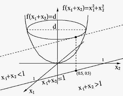
Example:
Find the extremum of
 subject to each of
the three different constraints:
subject to each of
the three different constraints:  ,
,
 , and
, and
 .
.
 |
 |
 |
 , i.e., the function
is minimized at
, i.e., the function
is minimized at
 . We note that
 and
and
 have the same gradients:
![$\displaystyle \bigtriangledown f(0.5,0.5)=\bigtriangledown h(0.5,0.5)=[1,1]^T$](img742.svg) |
 |
 and
and  .
According to Table 188, is
the solution for the minimization problem subject to
(left), or the maximization problem
subject to
.
.
According to Table 188, is
the solution for the minimization problem subject to
(left), or the maximization problem
subject to
.
 |
, and .
According to Table 188, is
not the solution of either the maximization problem
subject to
(left), or the minimization
problem subject to
(right), i.e., the
constraint is inactive. We therefore need to assume
and solve the following equations for an unconstrained problem:
 |
 and
and
 , with
minimum
, with
minimum
 . This is the solution for the
minimization problem (right), at which
,
i.e., the constraint is inactive. However this is not
the solution for the maximization problem (left) as the
function is not bounded from above.
. This is the solution for the
minimization problem (right), at which
,
i.e., the constraint is inactive. However this is not
the solution for the maximization problem (left) as the
function is not bounded from above.


