Spatial averaging (low-pass filtering)

The isolated pixels with gray values much different from its neighbors can be considered as impulses corresponding to high spatial frequencies. One way to get rid of this kind of noise is to use the average of a small local region in the image so that the out-of-range gray levels can be suppressed. Equivalently, this averaging operation in spatial domain corresponds to low-pass filtering in the spatial frequency domain.

The averaging operation is a weighted sum of the pixels in a small neighborhood and can be implemented by a common convolution with a kernel $w$ of certain shapes and values:

$$y[m,n]=\sum \sum_{i,j \in w} w[i,j]\;x[m-i,n-j] =\sum \sum_{i,j \in w} w[i,j]\;x[m+i,n+j]$$

where $w[i,j]=w[-i,-i]$ is a symmetric kernel of a limited size (typically 3x3, 5x5, 7x7, etc.). Some common kernels:

• 
  
  $$w=\frac{1}{4}\left[ \begin{array}{cc} 1 & 1 1 & 1 \end{array} \right]$$
  
  

• 
  
  $$w=\frac{1}{6}\left[ \begin{array}{ccc} 0 & 1 & 0 1 & 2 & 1 \\ 0 & 1 & 0 \end{array} \right]$$
  
  

• 
  
  $$w=\frac{1}{9}\left[ \begin{array}{ccc} 1 & 1 & 1 1 & 1 & 1 \\ 1 & 1 & 1 \end{array} \right]$$
  
  

• 
  
  $$w=\frac{1}{10}\left[ \begin{array}{ccc} 1 & 1 & 1 1 & 2 & 1 \\ 1 & 1 & 1 \end{array} \right]$$
  
  

• 
  
  $$w=\frac{1}{16}\left[ \begin{array}{ccc} 1 & 2 & 1 2 & 4 & 2 \\ 1 & 2 & 1 \end{array} \right]$$
  
  

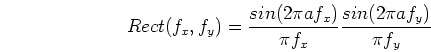
These convolution kernels can be considered as the approximations of some continuous 2D functions such as a rectangular function

$$rect(x,y)=\left\{ \begin{array}{ll} 1 & \mbox{if $\vert x\v... ...and $\vert y\vert<b$} \\ 0 & \mbox{else} \end{array} \right.$$

and a Gaussian function

$$gauss(x,y)=e^{-\frac{x^2+y^2}{2\sigma^2}}$$

Convolution with such functions in spatial domain $(x,y)$ is equivalent to the filtering in spatial frequency domain $(f_x,f_y)$ with the Fourier transforms of the kernel functions:

$$Rect(f_x,f_y)=\frac{sin(2\pi a f_x)}{\pi f_x}\frac{sin(2\pi a f_y)}{\pi f_y}$$

and

$$Gauss(f_x,f_y)=\sqrt{2\pi\sigma^2}e^{-\frac{\sigma^2(\omega_x^2+\omega_y^2)}{2}}$$

In general the Gaussian function is a preferred method for the following reasons:

• Rotational symmetric with no bias on any particular direction;
• Closer neighbors contribute more (larger weights) than those farther away;
• The width of the function can be easily controlled;
• Fourier transform of Gaussian is also Gaussian so that the filtering in frequency domain is smooth.

Weymouth-Overton's algorithm

• Define weights for each pixel $x[i,j]$ in the neighborhood W of the pixel $x[m,n]$ under consideration. The distance weight is defined as:
  
  $$w_d[i,j]=\frac{1}{1+\sqrt{(m-i)^2+(n-j)^2}$$
  
  
  and the value weight is defined as:
  
  $$w_v[i,j]=\frac{1}{1+[x[i,j]-x[m,n]]^\alpha}$$
  
  
  where $\alpha$ is a user specified parameter. The overall weight for pixel $x[i,j]$ is defined as
  
  $$w[i,j]=w_d[i,j]\; w_v[i,j]$$
  
  
  Pixels close to $x[m,n]$ in both distance and value will have larger weights.

• Replace $x[m,n]$ by
  
  $$y[m,n]=\frac{\sum_{(i,j)\in W} w[i,j] x[i,j]}{\sum_{(i,j)\in W} w[i,j] }$$