Summary of BP training

The following is for one randomly chosen training pattern pair $\{{\bf x}_p, {\bf y}_p\}$.

1. Apply ${\bf x}_p=[x_{p1}, x_{p2}, ... , x_{pn}]^T$ to the input nodes;

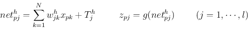
2. Compute net input to and output from all nodes in the hidden layer:
   
   $$net^h_{pj}=\sum_{k=1}^N w_{jk}^{h} x_{pk}+T^h_j\;\;\;\;\;\;\;\;\; z_{pj}=g(net^h_{pj})\;\;\;\;\;\;\;\;(j=1,\cdots,l)$$
   
   

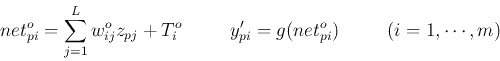
3. Compute net input to and output from all nodes in the output layer:
   
   $$net^o_{pi}=\sum_{j=1}^L w_{ij}^{o} z_{pj} + T^o_i\;\;\;\;\;\;\;\;\; y'_{pi}=g(net^o_{pi})\;\;\;\;\;\;\;\;\;(i=1,\cdots,m)$$
   
   

4. Compare the output $y'_{pi}$ with the desired output ${\bf y}_p=[y_{p1},y_{p2},...,y_{pm}]^T$ corresponding to the input ${\bf x}_p$, to find the error terms for all output nodes (not quite the same as defined previously):
   
   $$\delta_{pi}^{o}=g'(net^o_{pi}) (y_{pi}-y'_{pi}) \;\;\;\;\;\;\;\;(i=1,\cdots,m)$$
   
   

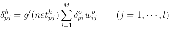
5. Find error terms for all hidden nodes (not quite the same as defined previously)
   
   $$\delta_{pj}^{h}=g'(net^h_{pj}) \sum_{i=1}^M \delta_{pi}^{o} w_{ij}^o \;\;\;\;\;\;\;(j=1,\cdots,l)$$
   
   

6. Update weights to output nodes
   
   $$w_{ij}^o \leftarrow w_{ij}^o+\eta \delta_{pi}^o z_{pj}\;\;\;\;\;\;\;(i=1,\cdots,m,\;\;j=1,\cdots,l)$$
   
   

7. Update weights to hidden nodes
   
   $$w_{jk}^h \leftarrow w_{jk}^h+\eta \delta_{pj}^h x_{pk}\;\;\;\;\;\;\;(j=1,\cdots,l,\;\;k=1,\cdots,n)$$
   
   

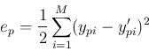
8. Compute
   
   $$e_p=\frac{1}{2}\sum_{i=1}^M (y_{pi}-y'_{pi})^2$$
   
   

This process is then repeated with another pair of $\{{\bf x}_p, {\bf y}_p\}$ in the training set. When the error is acceptably small for all of the training pattern pairs, training can be terminated.

The training process of BP network can be considered as a data modeling problem:

$${\bf y}_p={\bf f}({\bf x}_p,{\bf w})$$

The goal is to find the optimal parameters, the weights of both the hidden and output layers, based on the observed dataset, the training data of $K$ pairs $\{ ( {\bf x}_p,{\bf y}_p), (p=1,\cdots,K)\}$. The Levenberg-Marquardt algorithm discussed previously can be used to obtain the parameters, such as Matlab function trainlm.

Applications of BP networks include:

• Pattern recognition/classification
• Medical diagnosis (symptoms, diagnosis, drugs)
• Time series analysis (curve-fitting, interpolation and extrapolation, e.g., stock-market prediction).
• Data compression
• Automation (robots, autonomous vehicles)
• .....

A story related (maybe) to neural networks

An elementary school teacher asked her class to give examples of the great technological inventions in the 20th century. One kid mentioned it was the telephone, as it would let you talk to someone far away. Another kid said it was the airplane, because an airplane could take you to anywhere in the world. Then the teacher saw little Johnny eagerly waving his hand in the back of the classroom. ``What do you think is the greatest invention, Johnny?'' ``The thermos!'' The teacher was very puzzled, ``Why do you think the thermos? All it can do is to keep hot things hot and cold things cold.'' ``But'', Johnny answered, `` how does it know when to keep things hot and when to keep them cold?''

Don't you sometimes wonder ``How does a neural network know ...?''

Well, it does not. It is just a monkey-see-monkey-do type of learning, like this...