First consider nonlinearly mapping all data points ![]() to
to
![]() in a higher dimensional feature space
in a higher dimensional feature space ![]() , where
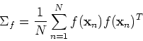
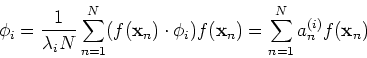
the covariance matrix can be estimated as
, where
the covariance matrix can be estimated as
![\begin{displaymath}[\frac{1}{N}\sum_{n=1}^N f({\bf x}_n) f({\bf x}_n)^T]\phi_i
=...
...}^N (f({\bf x}_n)\cdot \phi_i) f({\bf x}_n)
=\lambda_i \phi_i \end{displaymath}](img36.png)
![\begin{displaymath}{\bf K}=\left[ \begin{array}{ccc} ...&...&...\\
...&k({\bf x}_i,{\bf x}_j)&... ...&...&...\end{array} \right]_{N\times N} \end{displaymath}](img45.png)
Any new data point ![]() can now be mapped to
can now be mapped to ![]() in the
high-dimensional space
in the
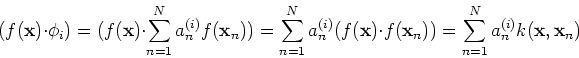
high-dimensional space ![]() , where its i-th PCA component can be
obtained as its projection on the i-th eigenvector
, where its i-th PCA component can be
obtained as its projection on the i-th eigenvector
![]()
These are the steps for the implementation of the kernel PCA algorithm:
Some commonly used kernels are:
The above discussion is based on the assumption that the data points have
zero mean, and therefore the covariance of two data points is the same as
their correlation. While the data points can be easily de-meaned in the
original space by subtracting the mean vector from all points, it is done
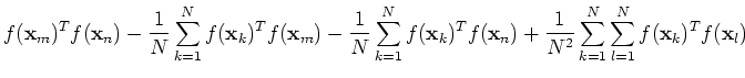
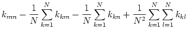
differently in the feature space. The de-meaned data points in the feature
space is:
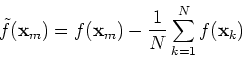
![$\displaystyle \tilde{f}({\bf x}_m)^T\tilde{f}({\bf x}_n)
=[f({\bf x}_m)-\frac{1...
...sum_{k=1}^N f({\bf x}_k)]^T
[f({\bf x}_n)-\frac{1}{N}\sum_{k=1}^N f({\bf x}_k)]$](img68.png) |
|||
 |
|||
 |
In summary, the mapping ![]() in the kernel PCA algorithm is never
explicitly specified, neither is the dimensionality of the feature space
in the kernel PCA algorithm is never
explicitly specified, neither is the dimensionality of the feature space
![]() . Similarly, the covariance matrix
. Similarly, the covariance matrix ![]() and its eigenvectors
and its eigenvectors
![]() are only mentioned in the above derivation, but they do not need to
be computed in implementation. The potential high dimensionality of
are only mentioned in the above derivation, but they do not need to
be computed in implementation. The potential high dimensionality of ![]() does not cost extra computation, as only the kernel
does not cost extra computation, as only the kernel
![]() is
needed in the implementation.
is
needed in the implementation.
Kernel PCA will have all the advantages of the regular PCA, as well as the
implicit nonlinear mapping to a feature space ![]() where the features
representing the structure in the data may be better extracted. For example,
data classification may be much more easily carried out in
where the features
representing the structure in the data may be better extracted. For example,
data classification may be much more easily carried out in ![]() due to
linear saparability.
due to
linear saparability.