Gaussian process

The function $f({\bf x},{\bf w})$ can be written as

$$f_n=\sum_{h=1}^H \phi_h({\bf x}^{(n)})\;(n=1,\cdots,N)\;\;\; \mbox{or in matrix form} \;\;\;{\bf f}={\bf\Phi} {\bf w}$$

If the prior distribution of the weights ${\bf w}$ is zero-mean Gaussian:

$$p({\bf w})=N(0,\Sigma_p)$$

then the function ${\bf f}({\bf w})$, as a linear function of ${\bf w}$, is also a zero-mean Gaussian:

$$p({\bf f})=N(0,{\bf Q})$$

where ${\bf Q}_{N\times N}$ is the covariancee matrix of ${\bf f}$:

$${\bf Q}=Cov({\bf f})=E({\bf ff}^T)=E({\bf\Phi w}({\bf\Phi w})... ...{\bf\Phi}E({\bf ww}^T){\bf\Phi}^T={\bf\Phi}\Sigma_p{\bf\Phi}^T$$

with the mn-th component being:

$$Q_{mn}=\phi^T({\bf x}^{(m)}) \Sigma_p \phi({\bf x}^{(n)}) =k({\bf x}^{(m)},{\bf x}^{(n)})$$

In particular, when $\Sigma_p=\sigma^2_p{\bf I}$, we get

$$Q_{mn}=\sigma^2_p \phi^T({\bf x}^{(m)}) \phi({\bf x}^{(n)}) ... ...ma^2_p \sum_{h=1}^H \phi_h({\bf x}^{(m)})\phi_h({\bf x}^{(n)})$$

The function $f$ is a Gaussian process as the distribution $p(f({\bf x}^{(1)}),\cdots,f({\bf x}^{(N)}))$ of any $N$ of its values correponding to $N$ input points is a Gaussian. As the noise $\epsilon \sim N(0,\sigma_n)$ is also a Gaussian distribution, the distribution of the $N$ values of the output $y=f({\bf x})+\epsilon$ are also Gaussian:

$${\bf y} \sim N(0,{\bf C})=N(0, {\bf Q}+\sigma_n^2{\bf I})$$

where ${\bf C}_{N\times N}$ is the covariance matrix of ${\bf y}$:

$${\bf C}={\bf Q}+\sigma_n^2{\bf I}={\bf\Phi}\Sigma_p{\bf\Phi}^T +\sigma_n^2{\bf I}$$

with the mn-th component being:

$$C_{mn}=k({\bf x}^{(m)},{\bf x}^{(n)})+\delta_{mn}\sigma_n^2$$

The result above can be generalized when $H \rightarrow \infty$, i.e., the function $f$ is expressed as the linear combination (integration rather than summation) of basis functions. For example, assume $d=1$ and the h-th basis is a radial function centered at $h$:

$$\phi_h(x^{(n)})=exp(-\frac{(x^{(n)}-h)^2}{2r^2})$$

and $\Sigma_p=\sigma_p{\bf I}$, the covariance $Q_{mn}$ becomes

$$Q_{mn} = Cov(x^{(m)}, x^{(n)})=\phi S\;\int_{-\infty}^{\infty} \phi_h(x^{(m)})\phi_h(x^{(n)})\; dh$$

$$= S\;\int_{-\infty}^{\infty} exp(-\frac{(x^{(m)}-h)^2}{2r^2}) exp(-\frac{(x^{(n)}-h)^2}{2r^2})\; dh$$

$$= S'\; exp(-\frac{(x^{(m)}-x^{(n)})^2}{4r^2})$$

where $S$ and $S'$ are some scaling factors (including $\sigma_p$). More generally, when $d>1$, the covariance matrix of the $N$ function values ${\bf f}$ at the $N$ input points ${\bf x}^n,\;(n=1,\cdots,N)$ can be defined as

$$Q_{mn}=k({\bf x}^{(m)},{\bf x}^{(n)}),\;\;\;\;(m,n=1,\cdots,N)$$

Now the regression problem can be approached based on a totally different point of view. Instead of specifying the basis functions and some model parameters (e.g. the weights ${\bf w}$), we can assume the $N$ function values ${\bf f}$ to be a Gaussian process and construct its covariance matrix (while always assume zeromean vector):

$$\Sigma_f={\bf Q}=Cov({\bf f})=\left[ \begin{array}{ccc}...&..... ......&...&...\end{array} \right]_{N\times N} =K({\bf X},{\bf X})$$

The mn-th component of the covariance matrix is

$$Q_{mn}=k({\bf x}^{(m)},{\bf x}^{(n)})$$

which be constructed according to the specific problem. For example, the following covariances can be used:

$$Q_{mn}=c\;exp(-\frac{({\bf x}^{(m)}-{\bf x}^{(n)})^T({\bf x}^{(m)}-{\bf x}^{(n)})}{2r^2})$$

$$Q_{mn}=c\;exp(-\frac{sin^2(\pi ({\bf x}^{(m)}-{\bf x}^{(n)})^T({\bf x}^{(m)}-{\bf x}^{(n)}))}{2r^2})$$

$$Q_{mn}=c\;exp(-\frac{({\bf x}^{(m)}-{\bf x}^{(n)})^T({\bf x}^{(m)}-{\bf x}^{(n)})}{2r^2})+x^{(m)}x^{(n)}$$

Comments:

• The motivation behind the general form of these covarances is the intuition that similar inputs (small $(x^{(m)}-x^{(n)}$) should give rise to similar predictions (large covarance or correlation $c_{mn}$).
• Here the covarance $Q_{mn}=k({\bf x}^{(m)},{\bf x}^{(n)})$ can be considered as some kernel function of the two vector arguments as used in various kernel-based algorithms such as support vector machine and kernel PCA. In either case, these kernels need to be constructed based on some prior knowledge of the problem.

For the output $y=f({\bf x})+\epsilon$, the covariance matrix becomes:

$$C_{mn}=Q_{mn}+\delta_n^2\delta_{mn},\;\;\;\;(m,n=1,\cdots,N) \;\;\;\;\mbox{or}\;\;\;\;{\bf C}={\bf Q}+\sigma_n {\bf I}$$

and its prior distribution is:

$$p({\bf y})=N(0,{\bf C})=\frac{1}{Z}e^{-\frac{1}{2}{\bf y}{\bf C}^{-1}{\bf y}}$$

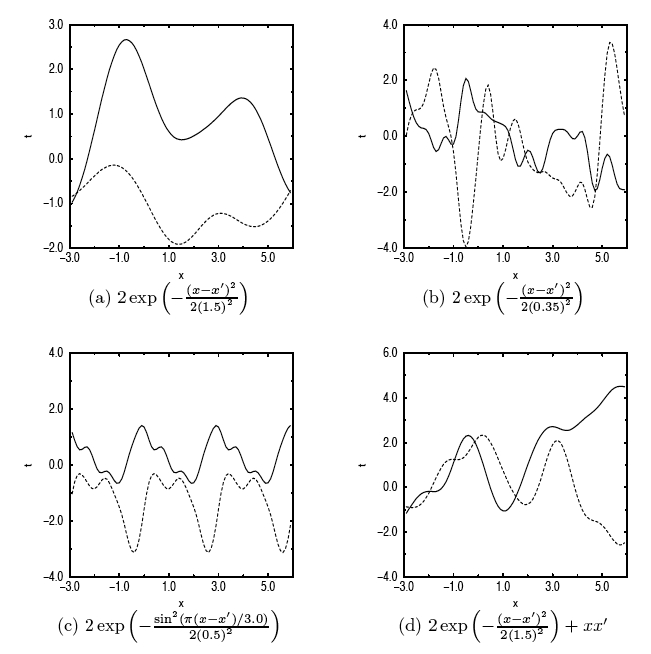
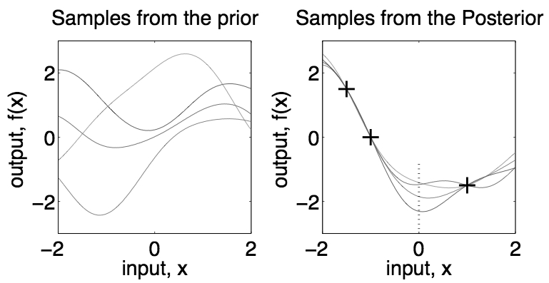
Samples from this distribution $N(0,{\bf C})$ can be drawn to get the $N$ values of the function $y$, i.e., various curves in 1-D space.

Now the regression problem of finding the underlying function $f({\bf x})$ to fit the observed data

$${\cal D}=({\bf X}, {\bf y})=\{ ({\bf x}^{(n)}, y^{(n)}), (n=1,\cdots,N)\}$$

is turned into a problem of finding the posterior distribution of the output:

$$p({\bf y}^*\vert{\bf X}^*,{\cal D})=p({\bf y}^*\vert{\bf X}^*... ... y}\vert{\bf X}^*,{\bf X})}{p({\bf y}\vert{\bf X}^*,{\bf X})}$$

As the function $f({\bf x})$ as well as output $y=f({\bf x})+\epsilon$ are Gaussian process, the conditional distribution of ${\bf y}^*$ given ${\bf y}$ can be found as below (proof given in Appendix A).

We first consider finding the conditional distribution of function values ${\bf f}^*$. Set up the function vector containing both the known values ${\bf f}$ and the prediction ${\bf f}^*$:

$$\left[ \begin{array}{c} {\bf f} {\bf f}^* \end{array} \right]$$

The normal distribution of this vector is determined by the mean vector (assumed to be zero) and the constructed covariance matrix, which is expressed in four blocks according to the dimensions (number of points) of ${\bf f}$ and ${\bf f}^*$:

$$\Sigma_f=Cov\left[ \begin{array}{c} {\bf f} {\bf f}^* \end... ...\bf X}^*,{\bf X}) & K({\bf X}^*,{\bf X}^*) \end{array} \right]$$

Now the conditional distribution of ${\bf f}^*$ given ${\bf f}$ can be found:

$$p({\bf y}^*\vert{\bf X}^*,{\bf X},{\bf y})=N(\mu_{(f^*\vert f)},\Sigma_{(f^*\vert f)})$$

where

$$\left\{ \begin{array}{l} \mu_{(f^*\vert f)}=K({\bf X},{\bf X}... ...({\bf X},{\bf X})^{-1}K({\bf X}^*,{\bf X}) \end{array} \right.$$

As the covariance matrix $K({\bf X},{\bf X})$ is symmetric, $K({\bf X}^*,{\bf X})^T=K({\bf X},{\bf X}^*)$.

If ${\bf Q}$ above is replaced by ${\bf C}={\bf Q}+\sigma_n{\bf I}$, the discussion is also valid for output ${\bf y}$.

The samples drawn from this posterior distribution $p({\bf y}^*\vert{\bf X}^*,{\cal D})=p({\bf y}^*\vert{\bf X}^*,{\bf X},{\bf y})$ are different curves that interpolate (fit) the observed data, the $N$ data points ${\cal D}=\{({\bf x}^{(n)},y^{(n)}), (n=1,\cdots,N) \}$, and they can also predict the outputs $y^*$ at any input points ${\bf x}^*$.

In summary, the regression problem can be approached in two different ways:

• The weight space view: the function is modeled as a linear combination of a set of $H$ discrete basis functions $\phi_h({\bf x})$ (could be just the $N$ input points ${\bf x}^{(n)}$ in the linear model), and a set of model parameters, the weights, is assumed. The covariance matrix of the function is
  
  $$Q_{mn}=k({\bf x}^{(m)},{\bf x}^{(n)}) =\sigma^2_p \sum_{h=1}^H \phi_h({\bf x}^{(m)})\phi_h({\bf x}^{(n)})$$
  
  

• The function space view: an infinite number of basis functions are taken from a function space, and no weights are specified. Instead, the convariance $Q_{mn}=k({\bf x}^{(m)},{\bf x}^{(n)})$ of the function (assumed a Gaussian process) can be constructed, so long as the resulting convariance matrix is positive definite.

These two views can be unified by the Mercer's theorem: a given positive definite covariance function can be decomposed as

$$Q_{mn}=k({\bf x}^{(m)},{\bf x}^{(n)})=\sum_{h=1}^\infty \lambda_n \phi_i({\bf x}^{(m)})\phi_i({\bf x}^{(n)})$$

where $\lambda_i$ and $\phi_i$ are the eigenvalues and eigenfunctions respectively:

$$\int k({\bf x}^{(m)},{\bf x}^{(n)})\phi_i({\bf x}^{(m)})d{\bf x}^{(m)} =\lambda_i \phi_i({\bf x}^{(n)})$$

In the weight space view, the covariance matrix is a result of the basis functions and their weights, while in the function space view, the covariance matrix is constructed first without explicitely specifying the basis functions and their weight.