Next: A 2D DFT Example Up: fourier Previous: Physical Meaning of 2DFT

Matrix Form of 2D DFT

Reconsider the 2D DFT:

$\begin{displaymath} X[k,l] = \frac{1}{\sqrt{MN}}\sum_{n=0}^{N-1} [ \sum_{m=0}^{... ... X'[k,n] e^{-j2\pi \frac{nl}{N} } \;\;\;\;(k=0,1,\cdots,M-1) \end{displaymath}$

where $0 \leq m,k \leq N-1,\;\;0 \leq n,l \leq N-1$ and

$\begin{displaymath}X'[k,n]\stackrel{\triangle}{=}\frac{1}{\sqrt{M}}\sum_{m=0}^{N-1}x[m,n]e^{-j2\pi \frac{mk}{M}} \;\;\;\;\;(n=0,1,\cdots,N-1) \end{displaymath}$

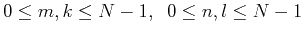
As the summation above is with respect to the row index

and the column index

can be treated as a fixed parameter, this expression can be considered as a one-dimensional Fourier transform of the nth column of

( $n=0,1,\cdots,N-1$ ), which can be written in column vector (vertical) form as:

$\begin{displaymath}{\bf X'}_n={\bf W}^*{\bf x}_n \end{displaymath}$

for all columns $n=0,\cdots,N-1$ . Putting all these

columns together, we can write

$\begin{displaymath}\left[{\bf X'}_0,\cdots,{\bf X'}_{N-1}\right]= {\bf W}^* \left[{\bf x}_0,\cdots,{\bf x}_{N-1}\right] \end{displaymath}$

or more concisely

$\begin{displaymath}{\bf X}' = {\bf W}^* {\bf x} \end{displaymath}$

where ${\bf W}^*$ is a

Fourier transform matrix.

We also note that the summation in the expression for is with respective to the column index n and the row index number k can be treated as a fixed parameter, the expression is one-dimensional Fourier transform of the kth row of ${\bf X}'$ , which can be written in row vector (horizontal) form as

$\begin{displaymath}{\bf X}_k^T=({\bf W}^* {\bf X'}_k)^T = {\bf X'}_k^T {\bf W}^{*T}, \;\;\;\;(k=0,\cdots,N-1) \end{displaymath}$

Putting all these

rows together, we can write

$\begin{displaymath}\left[ \begin{array}{c} {\bf X}_0^T . . {\bf X}_{N-1}... ...^T . . {\bf X}'_{N-1}^T \end{array} \right] {\bf W}^* \end{displaymath}$

( ${\bf W}$ is symmetric: ${\bf W}^{*T}={\bf W}^*$ ), or more concisely

$\begin{displaymath}{\bf X}={\bf X}'{\bf W}^* \end{displaymath}$

But since ${\bf X}' ={\bf W}^* {\bf x}$ , we have

$\begin{displaymath}{\bf X}={\bf W}^* {\bf x} {\bf W}^* \end{displaymath}$

This transform expression indicates that 2D DFT can be implemented by transforming all the rows of ${\bf x}$ and then transforming all the columns of the resulting matrix. The order of the row and column transforms is not important.

Similarly, the inverse 2D DFT can be written as

$\begin{displaymath}{\bf x}= {\bf W} {\bf X} {\bf W} \end{displaymath}$

Again note that ${\bf W}$ is a symmetric Unitary matrix:

$\begin{displaymath}{\bf W}^{-1}={\bf W}^{*T}={\bf W}^* \end{displaymath}$

It is obvious that the complexity of 2D DFT is which can be reduced to 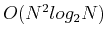if FFT is used.

Next: A 2D DFT Example Up: fourier Previous: Physical Meaning of 2DFT

Ruye Wang 2009-12-31