Histogram Specification

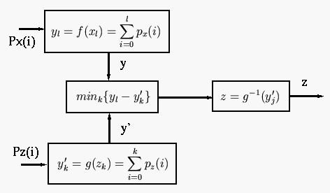
Here we want to convert the image so that it has a particular histogram that can be arbitrarily specified. Such a mapping function can be found in three steps:

• Equalize the histogram of the input image
• Equalize the specified histogram
• Relate the two equalized histograms

We first equalize the histogram $p_x$ of the input image $x$:

$$y=f(x)=\int_0^x p_x(u) du$$

We then equalize the desired histogram $p_z$ of the output image $z$:

$$y'=g(z)=\int_0^z p_z(u) du$$

The inverse of the above transform is

$$z=g^{-1}(y')$$

As the two intermediate images $y$ and $y'$ both have the same equalized histogram, they are actually the same image, i.e., $y=y'$, and the overall transform from the given image $x$ to the desired image $z$ can be found to be:

$$z=g^{-1}(y')=g^{-1}(y)=g^{-1}(f(x))$$

However, as the image gray levels are discrete, the continuous mapping obtained above can only be approximated. The discrete histograms $h_y[i]$ and $h_{y'}[i]$ are not necessarily identical. We therefore need to relate each gray level in $x$ with $h_x[i]\ne 0$ to a gray level in $z$ with $h_z[j]\ne 0$, so that the mapping from $y$ to $y'$ can be established.

Here are the steps of the algorithm:

• Step 1: Find histogram of input image $h_x$, and find its cumulative $H_x$, the histogram equalization mapping function:
  
  $$H_x[j]=\sum_{i=0}^j h_x[i]$$
  
  

• Step 2: Specify the desired histogram $h_z$, and find its cumulative $H_z$, the histogram equalization mapping function:
  
  $$H_z[j]=\sum_{i=0}^j h_z[i]$$
  
  

• Step 3: Relate the two mapping above to build a lookup table for the over all mapping. Specifically, for each input level $i$, find an output level $j$ so that $H_z[j]$ best matches $H_x[i]$:
  
  $$\vert H_x[i]-H_z[j] \vert = min_k \vert H_x[i]-H_z[k] \vert$$
  
  
  and then we setup a lookup entry $lookup[i]=j$.

Example:

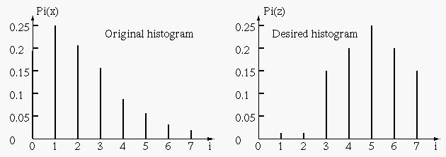
The histogram of the given image and the histogram desired are shown below:

• Step 1: Equalize $p_x$ to get mapping $y=f(x)$ (save as previous example).

  $x_i$	$n_j$	$h_x$	$y=H_x$
  0	790	0.19	0.19
  1	1023	0.25	0.44
  2	850	0.21	0.65
  3	656	0.16	0.81
  4	329	0.08	0.89
  5	245	0.06	0.95
  6	122	0.03	0.98
  7	81	0.02	1.00

• Step 2: Equalize $p_z$ to get mapping $y'=g(z)$.

  $z_i$	$p_z$	$y'=H_z$
  0	0.0	0.0
  1	0.0	0.0
  2	0.0	0.0
  3	0.15	0.15
  4	0.20	0.35
  5	0.30	0.65
  6	0.20	0.85
  7	0.15	1.0

• Step 3: Obtain overall mapping, $x \rightarrow y \rightarrow y' \rightarrow z$

  $x_i=i$	$y_j=H_x$	$y'_j=H_z$	$z_j=j$
  0	0.19	0.0	3
  1	0.44	0.0	4
  2	0.65	0.0	5
  3	0.81	0.15	6
  4	0.89	0.35	6
  5	0.95	0.65	7
  6	0.98	0.85	7
  7	1.0	1.0	7

  Here is the look-up table:

  i	0	1	2	3	4	5	6	7
  j	3	4	5	6	6	7	7	7

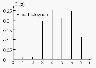
  This is the histogram of the resulting image:

  

In the following example, the desired histogram is a triangle with linear increase in the lower half of the the gray level range, and linear decrease in the upper half. Again the cumulative histogram shows indeed the density histogram is such a triangle.