Gray level mapping

Histogram:

In a typical 8-bit image, there are $L=2^8=256$ discrete gray scale levels from 0 to $2^8-1=255=L-1$. The histogram of an image represents the density probability distribution of the pixel values in the image over the entire gray scale range. The ith entry of the histogram is $h[i]=n_i/M/N$ ( $i=0,\cdots, L-1=255$) for the probability of a randomly chosen pixel to have the gray level $i$, where $n_i$ is the number of pixels of gray level $i$ in an image of size $M\times N$. Given $h[i]$, we can also find the cumulative distribution function:

$$H[j]=\sum_{i=0}^j h[i],\;\;\;\;\;\;\;(j=0,\cdots,L-1)$$

We obviously have

$$H[L-1]=\sum_{i=0}^{L-1} h[i]=1$$

Both the density and cumulative distribution functions $h$ and $H$ can be displayed graphically as an image.

Gray level mapping:

The appearance (brightness, contrast, etc.) of an image can be modified according to various needs by a gray level mapping function specified by the user:

$$y=f(x)$$

where $x=x[m,n]$ is a pixel in the input image and $y=y[m,n]$ is the corresponding pixel in the output image. This mapping function can be specified in different ways, such as a piecewise linear function, or based on the histogram of the input image.

Programming issues:

The above mapping functions can be carried out for each of the pixels in the image. However, this is not the most efficient way computationally. A better way for implementing the function mapping is to use a lookup table which stores the pre-computed mapping for each of the $L$ gray levels. The gray level of a pixel in the input image is used as the address to the table and the content of the table entry is used as the gray level of the corresponding pixel of the output image. By using the lookup table, the mapping function only needs to be carried out $L$ times, instead of $M\times N$ ($» L$) times (size of the image).

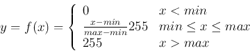
Common mapping functions:

Here are some common gray scale mapping functions $y=f(x)$:

• Thresholding:

  

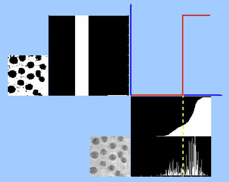
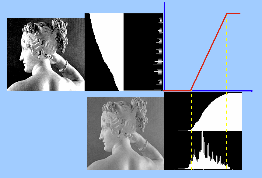
  As a special case of piecewise linear mapping, thresholding is a simple way to do image segmentation, in particular, when the histogram of the image is bimodal with two peaks separated by a valley, typically corresponding to some object in the image and the background. A thresholding mapping maps all pixel values below a specified threshold to zero and all above to 255.

  

• Negative image:
  
  $$y=f(x)=255-x$$
  
  
  This mapping is shown below which generates the negative of the input image:

  

• Min-max linear stretch:

  

  
  

  $$y=f(x)=\left\{ \begin{array}{ll} 0 & x<min \\ \frac{x-min}{... ... 255 & min \le x \le max \\ 255 & x>max \end{array} \right.$$
  
  
  This is a piecewise linear mapping between the input and output images of three linear segments with slopes 0 for $x<min$, $255/(max-min)>1$ for $min \le x \le max$, and 0 for $x>max$. The greater than 1 slope in the middle range stretches the dynamic range of the image to use all gray levels available in the display.

  

• Linear stretch based on histogram:

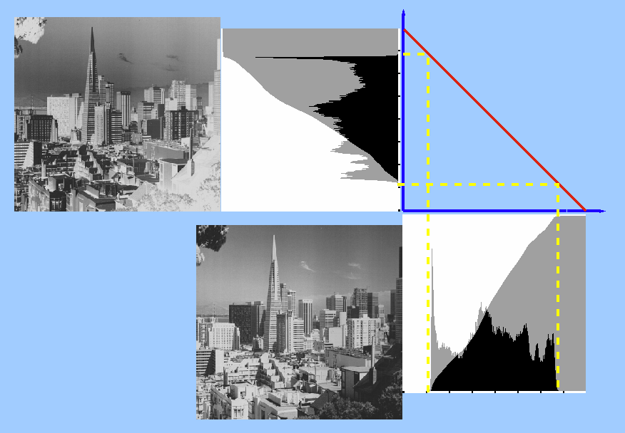
  If in the image there are only a small number of pixels close to minimum gray level 0 and the maximum gray level $L-1=255$, and the gray level of most of the pixels are concentrated in the middle range (gray) of the histogram, the above linear stretch method based on the minimum and maximum gray levels has very limited effect (as the slope $(L-1)/(max-min)$ is very close to 1).

  In this case we can push a small percentage (e.g., $3\%$, $5\%$) of gray levels at the two ends of the histogram toward 0 and $L-1$.

  

  

• Piecewise linear mapping:

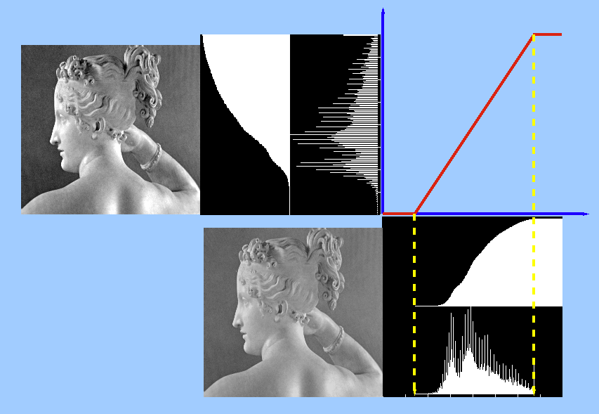
  A mapping function can be specified by a set of $n$ break-points $(x_i,y_j), i=1,2,\cdots,n$, with neighboring points connected by straight lines, such as shown here:

  

  For example, to increase the contrast of the image of Paolina, we can linearly stretch the gray scales of the image so that the darkest and brightest gray levels are mapped to 0 and 255, respectively.

Code Segments:

• Histogram: Here $h[i]$ and $H[i]$ are the density and cumulative distribution functions.

  
  

  $$\par \; for\; (i=0;\;i<L;\;i++)\; \{ \par \;\;\;\; h[i]=0;\;... ...or\; (i=1;\;i<L;\;i++)\; \par \;\;\;\; H[i]=H[i-1]+h[i]; \par$$
  
  

• Find cut-off levels:

  Assume $cut\_low$ and $cut\_high$ are fractions such as $3\%=0.03$ or $5\%=0.05$.

  
  

  $$\par \; w=0; \;\;min=0; \par \; while\; (w<cut\_low) \par \;... ...par \; while\; (w<cut\_high) \par \;\;\;\;\; w+=h[max--]; \par$$
  
  

• Build lookup table:

  
  

  $$\par \; slope=(L-1)/(max-min); \par \; for \;(i=0; \;i<L; \;... ...up[i]=L-1; \par \; \;\; else\;\; lookup[i]=slope*(i-min); \par$$
  
  

• Obtain output:

  
  

  $$\par \; for\;(i=0;\;i<M;\; i++) \par \; \;\;for\;(j=0;\; j<N;\; j++) \par \; \;\;\;\; y[i][j]=lookup[x[i][j]]; \par$$