Next: Reflection and termination
Up: transmission_line
Previous: transmission_line
As shown in the figure, a transmission line can be modeled by its
resistance and inductance in series, and the conductance and capacitance
in parallel, all distributed along its length in  direction. Here
  ,
,
 ,
,  and
and  represent, respectively, the resistance, inductance,
conductance, and capacitance per unit length
(
represent, respectively, the resistance, inductance,
conductance, and capacitance per unit length
(
![$[ohm]/[meter],\;[siemens]/[meter],\;[henry]/[meter],\;[farad]/[meter] $](img6.png) ).
).

The voltage  and current
  along the transmission line are
functions of both time variable
along the transmission line are
functions of both time variable  and space variable . Across an
infinitesimal section
and space variable . Across an
infinitesimal section  along the line, the voltage and current
changes are
along the line, the voltage and current
changes are
Dividing both sides of these equations by and let
 we get the telegrapher's equations:
These coupled partial differential equations (PDEs) of two variables and
, called the telegrapher's equations, can be more conveniently solved by
the Fourier transform method. We denote the Fourier transforms of the voltage
and current with respect of ( treated as a parameter) as
For convenience we may sometimes denote the voltage  and current
 in the Fourier domain as
  and
and  or simply
  and
and  .
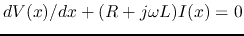
Taking the Fourier transform on both sides of the two PDEs we get two ordinary
differential equations (ODEs) with respect to a single variable :
.
Taking the Fourier transform on both sides of the two PDEs we get two ordinary
differential equations (ODEs) with respect to a single variable :
These ODEs can also be obtained when both voltage and current
are represented respectively as phasors and , and the transmission
line is represented in terms of the impedances , ,  , and
, and
 . Therefore the variables and in the ODEs can be
considered as either the Fourier transform or the phasor representations of
the voltage and current .
. Therefore the variables and in the ODEs can be
considered as either the Fourier transform or the phasor representations of
the voltage and current .
Combining the two equations we get
where we have defined
with
and
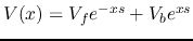
The solutions of these two second order ODEs can be found to be:
where we have defined
Here  and
and  are the two particular solutions, weighted by
the arbitrary constants
are the two particular solutions, weighted by
the arbitrary constants  and
and  , which are to be determined based
on the boundary conditions
, which are to be determined based
on the boundary conditions
![$V(0)={\cal F}[v(0,t)]$](img34.png) at the front and
at the front and
![$V(l)={\cal F}[v(l,t)]$](img35.png) at the back end of the transmission line of length
at the back end of the transmission line of length
 . Note that and are constants with respect to variable ,
but in time domain, they are still functions of variable . Constant
. Note that and are constants with respect to variable ,
but in time domain, they are still functions of variable . Constant  and
and  can be found the same way.
Substituting
 into the equation
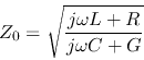
 and solving for , we get
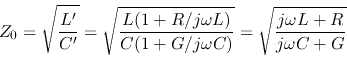
where
is the characteristic impedance of the transmission line measured in ohm.
Comparing the two expressions of above, we see that
Lossless transmission line
When the frequency  is high,
  and
and  are much
greater than and , we can assume the transmission line is loss-less
with
are much
greater than and , we can assume the transmission line is loss-less
with  . In this case the two ODEs above become
and we also have
where  the transmission speed (measued in meter/second) defined as
and
The voltage and current in time domain can be obtained as the inverse Fourier
transforms of
 and
and
 :
:
and
where
Both and are composed of two components traveling at velocity
in opposite directions along the transmission line. The time for the wave
to travel the whole length of the transmission line is  . At the
front (
. At the
front ( ) and back (
 ) ends of the line we have
i.e., the coefficients and are just the forward and backward
voltages at the front of the line ():
Lossy transmission line
When the signal frequency is low, and can no longer be assumed as
zero and the signal is always attenuated due to the resistance in serie
with the inductance and the leakage conductance in parallel with the
capacitance . The two first order ODEs can be written as
where we have defined
As the above equations take the same form as in the loss-less case (with
and replaced by  and
and  , respectively), it can be solved in the
same way. Now we have
, respectively), it can be solved in the
same way. Now we have
and
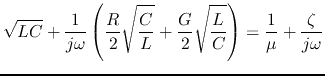
which can be approximated as below when  ,
,  :
:
The second approximation is due to the Taylor series:
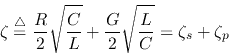
Here we have defined the attenuation constant or damping coefficient
as
which is simply the sum of the damping coefficient  of the
series RCL circuit and the damping coefficient
of the
series RCL circuit and the damping coefficient  of the parallel
GCL circuit:
of the parallel
GCL circuit:
As before, the solution of the above equations is
In the time domain we have
Note that the forward wave  attenuates exponentially as increases
from 0 to , while the backward wave
attenuates exponentially as increases
from 0 to , while the backward wave  attenuates exponentially as
decreases from to 0.
attenuates exponentially as
decreases from to 0.
Next: Reflection and termination
Up: transmission_line
Previous: transmission_line
Ruye Wang
2016-05-20
![\begin{displaymath}I(x)=-\frac{1}{j\omega L+R}\frac{dV(x)}{dx}
=\frac{s}{(j\ome...
... e^{-xs}-V_b e^{xs}]
=\frac{1}{Z_0}\;[V_f e^{-xs}-V_b e^{xs}]
\end{displaymath}](img41.png)
![\begin{displaymath}\sqrt{L'C'}=\sqrt{LC}\left[ \left(1+\frac{R}{j\omega L}\right)
\left(1+\frac{G}{j\omega C}\right) \right]^{1/2} \end{displaymath}](img71.png)
![$\displaystyle \sqrt{LC}\left(1+\frac{R}{j\omega L}+\frac{G}{j\omega C}\right)^{...
...}\left[1+\frac{1}{2}\left(\frac{R}{j\omega L}+\frac{G}{j\omega C}\right)\right]$](img76.png)