Bode Plots of Components

1. Constant gain $k$
     $$\left\{ \begin{array}{l} \mbox{If $k>0, \;\;\;\;k=\vert k\vert e... ..., \;\;Lm\;k=20\;\log_{10}\vert k\vert,\;\;\angle k=\pi$} \end{array} \right.$$ (143)

2. Delay factor: $e^{\pm j\omega \tau}$
     $$Lm \;e^{ j\omega \tau}=20\;\log_{10} \vert e^{ j\omega \tau}\vert=20\;\log_{10} 1=0,\;\;\;\; \angle e^{ j\omega \tau} =\pm \omega \tau$$ (144)

3. Derivative factor $j\omega=\omega\; e^{j\pi/2}$:
     $$Lm\; (j\omega)=20\; log_{10} \omega\;dB,\;\;\;\;\;\angle(j\omega)=\frac{\pi}{2}$$ (145)
   In particular:
   • When $\omega=1$, $Lm \;(1) =20\; \log_{10} 1=0\;dB$
   • If a frequency $\omega$ becomes ten times higher, then
       $$Lm\; (j10\omega)=20\; \log_{10} 10\omega=20 \;\log_{10} 10+20\;\log_{10}\omega =20+Lm(j\omega)$$ (146)
     The Lm plot of $j\omega$ is a straight line with a slop of 20 dB/dec that goes through a zero-crossing at $\omega=1$.

   Also consider two additional cases related to $j\omega$. First, $(j\omega)^{\pm m}=\omega^{\pm m} e^{\pm j m\pi/2}$

     $$Lm(j\omega)^{\pm m}=\pm m\;Lm(j\omega),\;\;\;\;\;\angle(j\omega)^{\pm m}=\pm m\pi/2$$ (147)
   The slop of the Lm plot is $\pm 20m/dec$. For example, when $m=2$, we have:
     $$Lm\; (j\omega)^2=40\log_{10}\omega,\;\;\;\;\;\angle\;(j\omega)^2=\pi$$ (148)

   Second, the plots of $j\omega\tau$ are similar to those of $j\omega$, except the zero-crossing occurs at $\omega\tau=1$, i.e., $\omega=1/\tau$.

4. Integral factor $1/j\omega=(j\omega)^{-1}$:
     $$Lm \;(j\omega)^{-1}=-Lm\;(j\omega)=-20\;log_{10} \omega\;dB, \;\;\;\;\angle\; (j\omega)^{-1}=-\angle(j\omega)=-\frac{\pi}{2}$$ (149)
   The Lm plot of $1/j\omega$ is a straight line with a slop of -20 dB/dec that goes through a zero-crossing at $\omega=1$.

5. First order factor in numerator $1+j\omega\tau$
     $$1+j\omega \tau=\sqrt{1+(\omega \tau)^2}\;e^{j\tan^{-1}(\omega \tau)} =\sqrt{1+(\omega \tau)^2}\;\angle \tan^{-1}(\omega \tau)$$ (150)
     $$Lm(1+j\omega \tau)=20\;\log_{10}\sqrt{1+(\omega \tau)^2} =20\;\log_{10}(1+(\omega \tau)^2)^{1/2}=10\;\log_{10}(1+(\omega \tau)^2)$$ (151)
     $$\angle(1+j\omega \tau)=\tan^{-1}(\omega\tau)$$ (152)
   Consider the following three cases:
   • $\omega\tau=1$, i.e., $\omega_c=1/\tau$ is the corner frequency, we have
       $$Lm(1+j)=20\;\log_{10} \sqrt{1^2+1^2}=20\;\log_{10} 0.707\approx 3.01\;dB,\;\;\;\;\; \angle(1+j)=\frac{\pi}{4}$$ (153)
   • $\omega\tau \ll 1$ (e.g., $\omega\tau\le 10$):
       $$Lm(1+j\omega \tau)\approx10\;\log_{10}(1)=0,\;\;\;\;\; \angle(1+j\omega \tau)\approx \angle(1)=0$$ (154)
   • $\omega\tau \gg 1$ (e.g., $\omega\tau\ge 10$):
       $$Lm(1+j\omega \tau)\approx 20\;\log_{10}(\omega \tau),\;\;\;\; \angle(1+j\omega \tau)\approx \angle(j\omega \tau)=\frac{\pi}{2}$$ (155)
   The straight-line asymptote of $Lm(1+j\omega\tau)$ has zero slope when $\omega\tau<1$ but a slope 20 dB/dec when $\omega\tau>1$. The straight-line asymptote of $\angle(1+j\omega\tau)$ is zero when $\omega\tau<0.1$, $\pi/2$ when $\omega\tau>10$, but with a slope $45^\circ/dec$ in between.

6. First order factor in denominator $1/(1+j\omega\tau)=(1+j\omega\tau)^{-1}$
     $$Lm\;(1+j\omega\tau)^{-1}=-Lm(1+j\omega\tau) =-10\;\log_{10}(1+(\omega \tau)^2)$$ (156)
     $$\angle\;(1+j\omega \tau)^{-1}=-\angle(1+j\omega \tau) =-\tan^{-1}(\omega\tau)$$ (157)
   Both the Lm and phase plots of $1/(1+j\omega\tau)$ is simply the negative version of $(1+j\omega\tau)$.

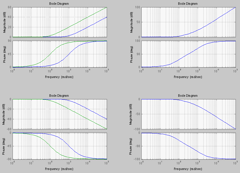
   The figure below shows the plots of two first order systems corner frequencies $\omega_1=100$ and $\omega_2=1000$, together with the plots of their product, a second order system.

   

7. Second-order factor
     $$H(j\omega)=\frac{1}{(j\omega)^2+2\zeta\omega_n j\omega+\omega_n^2... ...}{\omega_n^2}}{1-(\frac{\omega}{\omega_n})^2+j\,2\zeta\frac{\omega}{\omega_n}}$$ (158)
   The denominator is a 2nd order polynomial for variable $j\omega$. Consider the following two cases:

   First, if $\Delta=b^2-4ac=(2\zeta\omega_n)^2-4\omega_n^2=4\omega^2_n(\zeta^2-1)\ge 0$ i.e., if $\zeta\ge 1$, the denominator has two real and negative roots:

     $$p_{1,2}=(-\zeta\pm\sqrt{\zeta^2-1})\omega_n < 0$$ (159)
   and $H(j\omega)$ can be written as a product of two first order FRFs:
     $$H(j\omega)=\frac{1}{(j\omega-p_1)(j\omega-p_2)} =\frac{1/p_1p_2... ...1}{1+j\omega\tau_1}\;\frac{\tau_2}{1+j\omega\tau_2} =H_1(j\omega)H_2(j\omega)$$ (160)
   where $\tau_1=-1/p_1>0$ and $\tau_2=-1/p_2>0$ are the two time constant of the two first order systems. Now the second order factor is the product of two first order factors and
     $$Lm\;(H_1 H_2)=Lm\; H_1+Lm\; H_2,\;\;\;\;\angle (H_1 H_2)=\angle H_1+\angle H_2$$ (161)
   with corner frequencies at $\omega_{c1}=1/\tau_1=p_1$ and $\omega_{c1}=1/\tau_2=p_2$.

   Second, if $0<\zeta<1$, i.e., the two roots are complex. We consider the numerator and the denominator separately. The numerator is just a constant with zero phase and log-magnitude of $20\log_{10} \omega_n^{-}2=-40\log_{10} \omega_n$. Next consider the rest of the function:

     $$\vert H(j\omega)\vert=[(1-(\frac{\omega}{\omega_n})^2)^2+(2\zeta\frac{\omega}{\omega_n})^2]^{-1/2}$$ (162)
   We have
   

   $$Lm\;H(j\omega)=20\log_{10} \vert H(j\omega)\vert =-10\;\log_{10}[\; (1-(\frac{\omega}{\omega_n})^2)^2+(2\zeta\frac{\omega}{\omega_n})^2\;]$$ (163)

     $$\angle H(j\omega)=-\tan^{-1}\frac{2\zeta\omega/\omega_n}{1-(\omega/\omega_n)^2}$$ (164)
   Consider three cases:
   • $\omega/\omega_n=1$: Now $H(j\omega)=1/j2\zeta=-j/2\zeta$ and
       $$Lm\;H(j\omega)=-20\;\log_{10} 2\zeta,\;\;\;\;\;\angle H(j\omega)=-\frac{\pi}{2}$$ (165)
   • $\omega/\omega_n\ll 1$, i.e., $\omega \ll \omega_n$:
       $$Lm\;H(j\omega) \approx -10\;\log_{10} (1)=0,\;\;\;\;\;\angle H(j\omega)=0^\circ$$ (166)
   • $\omega/\omega_n\gg 1$, i.e., $\omega \ll \omega_n$:
       $$Lm\;H(j\omega)\approx-10\;\log_{10}[\; (\frac{\omega}{\omega_n})^4 ] =-40 \;\log_{10} \frac{\omega}{\omega_n}$$ (167)
     This is a straight line with slop of -40 dB per decade.
       $$\angle H(j\omega) \approx -\tan^{-1} (-2\zeta \omega_n/\omega) \approx -\tan^{-1} (-0)=-\pi=-180^\circ$$ (168)

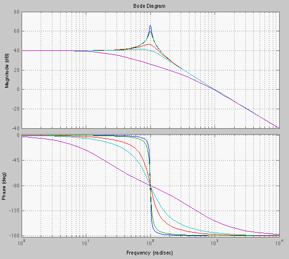
The magnitude of the second-order factor is

  $$\vert H(j\omega)\vert =\frac{1}{\sqrt{(1-\frac{\omega^2}{\omega_... ...2+4\zeta^2 \frac{\omega^2}{\omega_n^2}}} =\frac{1}{\sqrt{(1-u)^2+4\zeta^2 u}}$$ (169)

where $u=(\omega/\omega_n)^2$. When $u=1$ i.e., $\omega=\omega_n$, we have

  $$\vert H(j\omega_n) \vert=\frac{1}{2\zeta}=Q$$ (170)

However, the peak of $\vert H(j\omega)\vert$ is not at $\omega_n$, but at the resonant frequency $\omega_p$, which can be found by taking derivative of the magnitude of the denominator with respect to $u$ and setting it to zero:

  $$\frac{d}{du}[u^2+(4\zeta^2-2)u+1]=2u+4\zeta^2-2=0$$ (171)

Solving it, we get:

  $$u=\frac{\omega^2}{\omega_n^2}=1-2\zeta^2,\;\;\;\mbox{i.e.,} \;\;\;\;\omega=\omega_n\sqrt{1-2\zeta^2} < \omega_n$$ (172)

At this peak frequency $\omega_p=\omega_n\sqrt{1-2\zeta^2}$, the peak is:

  $$\vert H(j\omega_p) \vert=\frac{1}{2\zeta\sqrt{1-\zeta^2}} > \frac{1}{2\zeta}=\vert H(j\omega_n) \vert$$ (173)

Note that if $\zeta^2>1/2$, i.e., $\zeta>0.707$, the result is complex indicating there is no peak.