Higher order systems

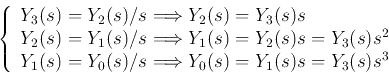
Higher than first order systems can be built with multiple integrators, as shown here for a third order system:

From the diagram, we can get

$$\left\{ \begin{array}{l} Y_3(s)=Y_2(s)/s \Longrightarrow Y_... ... \Longrightarrow Y_0(s)=Y_1(s)s=Y_3(s)s^3 \end{array} \right.$$

But we also have

$$Y_0(s)=X(s)-(k_1Y_1(s)+k_2Y_2(s)+k_3Y_3(s))$$

i.e.,

$$X(s)=Y_0(s)+k_1Y_1(s)+k_2Y_2(s)+k_3Y_3(s)=(s^3+k_1s^2+k_2s+k_3) Y_3(s)$$

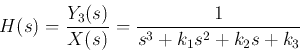
we get the transfer function

$$H(s)=\frac{Y_3(s)}{X(s)}=\frac{1}{s^3+k_1s^2+k_2s+k_3}$$

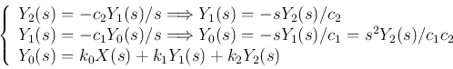
Second order system by 2 integrators

From the diagram, we can get

$$\left\{ \begin{array}{ll} Y_2(s)=-c_2Y_1(s)/s \Longrightarr... ...\\ Y_0(s)=k_0 X(s)+k_1Y_1(s)+k_2Y_2(s) \end{array} \right.$$

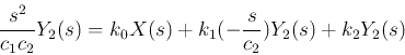
substituting the first two equations into the last one, we get

$$\frac{s^2}{c_1c_2} Y_2(s)=k_0X(s)+k_1(-\frac{s}{c_2})Y_2(s)+k_2Y_2(s)$$

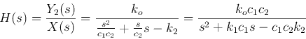
from which we obtain the transfer function as

$$H(s)=\frac{Y_2(s)}{X(s)}=\frac{k_o}{\frac{s^2}{c_1c_2}+\frac{s}{c_2}s-k_2} =\frac{k_oc_1c_2}{s^2+k_1c_1s-c_1c_2k_2}$$

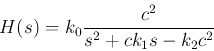
which is a second order system. In particular, if $c_1=c_2=c$, we have

$$H(s)=k_0\frac{c^2}{s^2+c k_1s-k_2c^2}$$

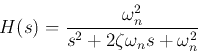
Comparing this with the canonical 2nd order system transfer function

$$H(s)=\frac{\omega_n^2}{s^2+2\zeta \omega_n s+\omega_n^2}$$

we see that we can let $c=\omega_n$ and $k_1=2\zeta$. Moreover, $k_2<0$, i.e., the feedback from the output should be negative. $k_0$ is a constant scalar which can take any value.