One-Way Analysis of Variance (ANOVA)

While the two-sample t-test (based on Student's t-distribution) tests whether two variables are the same, the one-way AVOVA (based on the F-distribution) tests whether $K\ge 3$ groups are the same. The null hypothesis is that all samples are drawn from populations with the same means. For example, we want to find out if any of the $K$ different treatments for a disease is on average superior or inferior to the others.

Specifically, let $\{C_1,\cdots,C_K\}$ be $K$ groups each containing $N_k$ samples $C_k=\{ x_1^{(k)},\cdots,x_{N_k}^{(k)}\}$. The total number of samples is $N=N_1+\cdots+N_K$. The null hypothesis is $H_0:\;\mu_1=\cdots=\mu_K$.

The method is based on the assumption that samples in each of the $K$ groups have normal distributions ${\cal N}(\mu_k,\sigma^2)$ of possibly different unknown means but the same unknown variance.

We first find the following

• Group means
    $$\bar{x}_k=\frac{1}{N_k}\sum_{x\in C_k} x,\;\;\;\;\;\;(k=1,\cdots,K)$$ (48)
• Total mean
    $$\bar{x}=\frac{1}{N}\sum_{\mbox{all $x$}} x =\sum_{k=1}^K\sum_{x\in C_k} x=\sum_{k=1}^K \frac{N_k}{N}\bar{x}_k =\sum_{k=1}^K p_k\bar{x}_k$$ (49)
  where $p_k=N_k/N$.
• Total sum of squares with $DFT=N-1$ degrees of freedom:
    $$SST=\sum_{\mbox{all $x$}} (x-\bar{x})^2 =\sum_{k=1}^K\sum_{x\in C_k} (x-\bar{x})^2$$ (50)
• Within-group sum of squares (error, unexplained) with $DFW=N-K$ degrees of freedom:
    $$SSW=\sum_{k=1}^K\sum_{x\in C_k} (x-\bar{x}_k)^2$$ (51)
• Between-group sum of squares (information, explained) with $DFB=K-1$ degrees of freedom:
    $$SSB=\sum_{k=1}^K N_k(\bar{x}_k-\bar{x})^2$$ (52)

We see that the three degrees of freedom the three sums of squares are similarly related by

  $$DFT=DFG+DFE,\;\;\;\;\;\;\;\;\;\;\;\;\;SST=SSW+SSB$$ (53)

While the first equation is obvious, the second equation can be proven below:

$$SST = \sum_{k=1}^K\sum_{x\in C_k} (x-\bar{x})^2 =\sum_{k=1}^K\sum_{x\in C_k}( x-\bar{x}_k+\bar{x}_k-\bar{x})^2$$

$$= \sum_{k=1}^K \sum_{{\bf x} \in C_k} [( x-\bar{x}_k)^2+2(x-\bar{x}_k)(\bar{x}_k-\bar{x})+(\bar{x}_k-\bar{x})^2]$$

$$= \sum_{k=1}^K \sum_{{\bf x} \in C_k} [( x-\bar{x}_k)^2+(\bar{x}_k-\bar{x})^2]=SSW+SSB$$ (54)

The last equality is due to the fact that the summation of the middle term is equal to zero. These sum of squares are measurements of variations (relative to the means) in the data set. While SST represents the total variation, SSB and SSW represent the variations from two difference sources, variation between the groups, directly related to the issue whether these groups have the same mean, and variation within each of the groups, treated as error.

We further define the following mean-squares (MS) of $\chi^2$ distributions

  $$MSG=\frac{SSB}{DFB}=\frac{SSB}{K-1},\;\;\;\;\;\; MSE=\frac{SSW}{DFW}=\frac{SSW}{N-K}$$ (55)

Now we can finally define the test statistic:

$$f = \frac{\mbox{signal}}{\mbox{error}} =\frac{\mbox{explained (between-group) variance}} {\mbox{unexplained (within-group) variance}}$$

$$= \frac{MSG}{MSE}=\frac{SSB/DFB}{SSW/DFW} \;\sim\;{\cal F}_{K-1,N-K}$$ (56)

which has a F-distribution with $K-1$ numerator d.f. and $N-K$ denominator d.f.

If all samples are drawn from the populations having the same means, SSB for between-group variation will be small and $f$ is likely to be less than 1. But if the samples are drawn from populations of different means, SSB will be larger than SSW for within-group variation, and $f$ is likely to be greater than 1. Also, if the sample size $N$ is large, i.e., there is a stronger evidence for different group means, then $f$ is large and $H_0$ is likely to be rejected.

Specifically, substituting the specific values obtained from the data set into the expression above, we get the value $f^*$ and the corresponding p-value from the F-distribution table (Matlab function 1-fcdf(f,DFG,DFE)), which are then compared with the critical value $f_\alpha$ corresponding to the given significant level $\alpha$ (Matlab function finv(1-alpha,DFG,DFE)). If $f^*>f_\alpha$, or equivalently $p<\alpha$, then we reject the null hypothesis $H_0$ and conclude that the $K$ means are significantly different. Otherwise, we accept $H_0$ as there is not significant evidence against it.

These can be summarized by the ANOVA table below:

  $$\begin{tabular}{l\vert\vert c\vert c\vert c\vert c\vert c\vert c}... ...FW & & & \\ \hline \mbox{Total} & SST & DFT=N-1 & & & & \\ \hline \end{tabular}$$ (57)

Example: Given $N_k=5$ samples of each of the $K=4$ groups below, find if their means are the same, $H_0: \mu_1=\mu_2=\mu_3=\mu_4$, for the significant level $\alpha=0.05$.

  $$\begin{tabular}{c\vert c\vert c\vert c}\hline Group 1 & Group 2 ... ... \hline 45 & 53 & 40 & 43 \\ \hline 44 & 45 & 37 & 36 \\ \hline \end{tabular}$$ (58)

The total number of samples is $N=20$, the degrees of freedom are

  $$DFG=K-1=3, \;\;\;\;\;DFE=N-K=16,\;\;\;\;DFT=N-1=19$$ (59)

The group means are:

  $$\bar{x}_1=49.4, \;\;\bar{x}_2=47.6,\;\;\;\bar{x}_3=39.2,\;\;\; \bar{x}_4=45.8$$ (60)

The total mean is $\bar{x}=45.5$. The sum of squares are

  $$SSB=297,\;\;SSW=382,\;\;SST=679$$ (61)

The value of the test statistic $f^*$ and the corresponding p-value are:

  $$f^*=\frac{SSB/DFB}{SSW/DFW}=\frac{297/3}{382/16} =4.147,\;\;\;\;\;\;p=0.024$$ (62)

This result is summarized in the table below:

  $$\begin{tabular}{c\vert c\vert c\vert c\vert c\vert c}\hline \mbo... ...39$\ \\ \hline SSW=382 & DFW=16 & 382/16=23.875 & & & \\ \hline \end{tabular}$$ (63)

As $f^*=4.147$ is greater than the critical value $f_\alpha=3.239$ corresponding to $\alpha=0.05$, and equivalently $p=0.024\;<\;\alpha=0.05$, the null hypothesis is rejected, i.e., the means of the $K=4$ groups are not the same.

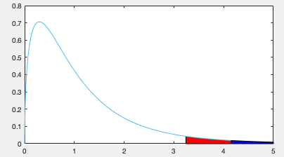
This result is also illustrated in the plot below, where the area to the right of $f_\alpha=3.239$ (red) is $\alpha=0.05$, while the area to the right of $f^*=4.147$ is $p=0.024$, which is inside the critical region, $H_0$ is rejected.