Linear Models of Illumination

Given the light received by the eye

$$L(\lambda)=R(\lambda) I(\lambda)$$

it is in general impossible to recover reflectance $R(\lambda)$ without knowing the illumination $I(\lambda)$. However, under certain conditions, it is possible to approximate both the reflectance and the illumination by some linear combination of a finite number of basis functions:

$$I(\lambda)\approx \sum_k e_k E_k(\lambda)$$

and

$$R(\lambda)\approx \sum_k f_k F_k(\lambda)$$

so that the error under some definition (e.g., squared-error) is minimized. For example, if squared error is used, we want

$$error\stackrel{\triangle}{=}[I(\lambda)-\sum_k e_k E_k(\lambda)]^2 \rightarrow min.$$

With these linear methods the task of recovering $r(\lambda)$ from $l(\lambda)$may become possible.

One example (Judd, Macadam, Wyszecki, 1964) is to approximate the power spectral distributions of daylight under various conditions. A large number (N=600) of daylight spectral distribution samples are collected at different times of day, under different weather conditions and on different continents.

The visible wavelength band (400 to 700 nm) is sampled at 10 nm interval so that each distribution is represented by n=31 numbers $\{x_i, \;(i=1,\cdots,n)\}$. And the distributions are normalized so that they are all equal to 100 at about the middle of the visible wavelength range $\lambda=560\; nm$. These N sample distributions can be considered as N=600 vectors of n=31 dimensions $\{ X_j,\;(j=1,\cdots,N)\}$, where $X_j=[x_{1j},\cdots,x_{nj}]^T$. Three of them are shown in the figure.

Then the principal component transform (PCT) is carried out to find a set of bases so that the various daylight distributions can be approximated by a linear combination of a small number of bases. Specifically, the PCT is carried out in the following steps:

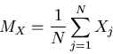
• Estimate the mean vector M_X of X_j's
  
  $$M_X=\frac{1}{N} \sum_{j=1}^N X_j$$
  
  

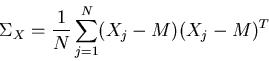
• Estimate the covariance matrix $\Sigma_X$ of X_j's
  
  $$\Sigma_X=\frac{1}{N} \sum_{j=1}^N (X_j-M)(X_j-M)^T$$
  
  

• Find eigenvalues $\{e_1,\cdots, e_n\}$ and eigenvectors $\{E_1,\cdots,E_n\}$ of the symmetric covariance matrix $\Sigma_X$ so that
  
  $$\Sigma_X E_i = e_i E_i\;\;\;\;\;(i=1,\cdots, n)$$
  
  
  Here the eigenvalues are in descending order (from the largest to smallest) and the corresponding eigenvectors are arranged accordingly (from the eigenvector corresponding to the largest eigenvalue to that corresponding to the smallest).

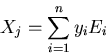
The n eigenvectors $\{E_1,\cdots,E_n\}$ so obtained are the bases so that each distribution X_j can be represented as the linear combination of them

$$X_j=\sum_{i=1}^n y_i E_i$$

where the coefficient y_i is the inner product of vectors X_j and E_i:

y_i=E_i^T X_j

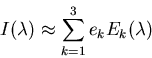
To use only a small number of the bases to approximate each distribution X_j, we truncate the above summation to keep only the first m<n terms (the principal components). It can be shown that the squared-error introduced by this truncation is equal to the sum of the eigenvalues corresponding to the those terms truncated. As the terms in the summation are arranged according to the descending order of the eigenvalues, we know the error is minimum. In fact, we can use as few as only m=3 terms to approximate all daylight distributions with insignificant errors.

$$I(\lambda)\approx \sum_{k=1}^3 e_k E_k(\lambda)$$

As shown in the figure, the first basis function happens to be the average of all daylight distributions, and the other two basis functions represent the short and long wavelength regions respectively.