Spatial averaging (low-pass filtering)

Image sensors and transmission channels may produce certain type of noise characterized by random and isolated pixels with out-of-range gray levels, which are either much lower or higher than the gray levels of the neighboring pixels. Such noise can be treated as some impulses corresponding to high spatial frequencies.

For example, digital photos taken under low illumination have low signal-to-noise ratio and are characterized by such random noisy pixels.

The challenge of suppressing and removing such noise is to distinguish between this type of isolated and out-of-range noise and other legitimate signal components such as the details, edges, lines, small features, etc. in the image, as both correspond to high frequency components in the image data, so that we can preserve the former while suppressing the latter.

One way to remove such noise is to replace each pixel by the average of the pixels in a small neighborhood so that the noise of out-of-range gray levels are reduced. Equivalently, this averaging operation in spatial domain corresponds to low-pass filtering in the spatial frequency domain, by which the high-frequency components are removed.

The averaging operation is a weighted sum of the pixels in a small neighborhood, typically of odd size in each dimension, i.e., $(2k+1)\times (2k+1)$ such as 3x3, 5x5, 7x7, although even-sized neighborhood can also be used. Such operation is typically implemented as a convolution with a symmetric kernel $w[m,n]=w[-m,-n]$ of certain shapes and values:

$$y[m,n] = \sum \sum_{-k\le i,j \le k} w[i,j]\;x[m-i,n-j] =\sum \sum_{-k\le i,j \le k} w[-i,-j]\;x[m+i,n+j]$$

$$= \sum \sum_{-k\le i,j \le k} w[i,j]\;x[m+i,n+j]$$ (1)

where $w[i,j]=w[-i,-i]$ is a symmetric kernel of a limited size (typically odd). Some common kernels are shown below:

$$w_1=\frac{1}{4}\left[ \begin{array}{cc} 1 & 1 \\ 1 & 1 \end{array... ...ft[ \begin{array}{ccc} 1 & 1 & 1 \\ 1 & 1 & 1 \\ 1 & 1 & 1 \end{array} \right]$$ (2)

$$w_4=\frac{1}{10}\left[ \begin{array}{ccc} 1 & 1 & 1 \\ 1 & 2 & 1 ... ...ft[ \begin{array}{ccc} 1 & 2 & 1 \\ 2 & 4 & 2 \\ 1 & 2 & 1 \end{array} \right]$$ (3)

The weighting of these convolution kernels is based on the assumption of spatial locality, i.e., the closer two pixels are, the more they are correlated. Consequently, closer neighbors of a pixel should be weighted more than those that are farther away.

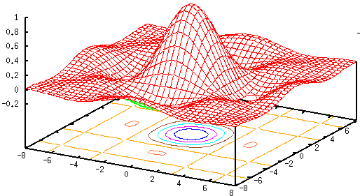
These convolution kernels can be considered as the approximations of some continuous 2D functions such as a rectangular function

$$rect(x,y)=\left\{ \begin{array}{ll} 1 & \mbox{if $\vert x\vert<a$\ and $\vert y\vert<b$} \\ 0 & \mbox{else} \end{array} \right.$$ (4)

and a Gaussian function

$$gauss(x,y)=e^{-\frac{x^2+y^2}{2\sigma^2}}$$ (5)

Convolution with such functions in spatial domain $(x,y)$ is equivalent to the filtering in spatial frequency domain $(f_x,f_y)$ with the Fourier transforms of the kernel functions:

$$Rect(f_x,f_y)=\frac{sin(2\pi a f_x)}{\pi f_x}\frac{sin(2\pi a f_y)}{\pi f_y}$$ (6)

and

$$Gauss(f_x,f_y)=\frac{1}{2\pi\sigma^2}e^{-\frac{(f_x^2+f_y^2)}{2\sigma^2}}$$ (7)

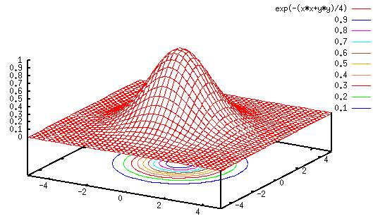
In general the Gaussian function is a preferred method for the following reasons:

• Rotational symmetric with no bias on any particular direction;
• Closer neighbors contribute more (larger weights) than those farther away;
• The width of the function can be easily controlled;
• Fourier transform of Gaussian is also Gaussian so that the filtering in frequency domain is also smooth.

The algorithms below represent various efforts made to distinguish noise components from legitimate signal components.

Weymouth-Overton's algorithm

This algorithm is based on the idea that in the averaging process, greater weight should be assigned to pixels that are

• closer to the pixel in question (in the center of the neighborhood) in distance, and
• more similar to the pixel in gray scale value.

as such a pixel is more relevant and its value is more reliable. Other pixels that are more different from the center pixel in both distance and gray scale value should be weighted less. Correspondingly the weight has two factors, $w_d$ for the distance and $w_v$ for the pixel value:

• Define weights for each pixel $x[i,j]$ in the neighborhood W of the pixel $x[m,n]$ under consideration. The distance weight is defined as:

  $$w_d[i,j]=\frac{1}{1+\sqrt{(m-i)^2+(n-j)^2}}$$ (8)

  and the value weight is defined as:

  $$w_v[i,j]=\frac{1}{1+[x[i,j]-x[m,n]]^\alpha}$$ (9)

  where $\alpha$ is a user specified parameter. The overall weight for pixel $x[i,j]$ is defined as

  $$w[i,j]=w_d[i,j]\; w_v[i,j]$$ (10)

  Pixels closer to $x[m,n]$ in both distance and gray scale value will be assigned larger weights.

• Replace $x[m,n]$ by

  $$y[m,n]=\frac{\sum_{(i,j)\in W} w[i,j] x[i,j]}{\sum_{(i,j)\in W} w[i,j] }$$ (11)

  where the denominator is for normalization.

Statistical thresholding

First find the mean $\mu$ and the variance $\sigma^2$ of all pixels in the neighborhood $W$ of a given pixel $x[m,n]$ of the input image:

$$\mu=\frac{1}{N} \sum_{(i,j) \in W} x[i,j]$$ (12)

$$\sigma^2=\frac{1}{N} \sum_{(i,j) \in W} [x[i,j]-\mu]^2$$ (13)

where $N$ is the number of pixels in the neighborhood $W$.

Then find the corresponding pixel for the output image:

$$y[m,n]=\left\{ \begin{array}{ll} x[m,n] & \mbox{if $\vert x[m,n]-\mu\vert < \sigma T$} \\ \mu & \mbox{else} \end{array} \right.$$ (14)

where $T$ is a user specified threshold value.

Nagao's algorithm

• Define a set of K neighborhoods around the pixel $x[m,n]$ under consideration, for example, the eight 3x3 neighborhoods in N, NE, E, SE, S, SW, W, and NW directions. The pixel $x[m,n]$ should be included as a corner in each of these neighborhoods.

• Find the mean $\mu_i$ and variance $\sigma_i^2$ for each of the K neighborhoods.

• Replace pixel$x[m,n]$ by the mean value of the neighborhood having the smallest $\sigma^2$ and therefore most reliable:

  $$y[m,n]=\mu_i, \;\;\;\;\; \;\;\;\;\; \sigma_i^2=min\{\sigma_1^2,\cdots,\sigma_K^2\}$$ (15)

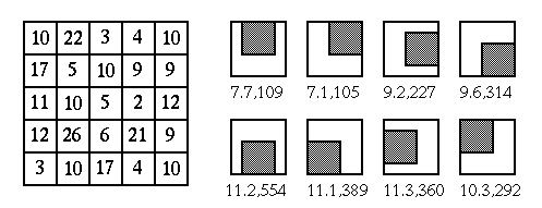
In this example, the pixel in question $x[m,n]=5$ is replaced by the mean 7.1 from the northeast neighborhood with minimum variance 105.