Geometric Interpretation of KLT

Assume the $N$ random variables in $X=[x_0,\cdots, x_{N-1}]^T$ have a normal joint probability density function:

$$p(x_0,\cdots, x_{N-1})=N(X, M_X, \Sigma_X)= \frac{1}{(2\pi)^... ...t\vert^{1/2}} exp[ -\frac{1}{2}(X-M_X)^T\Sigma_X^{-1}(X-M_X)]$$

where $M_X$ and $\Sigma_X$ are the mean vector and covariance matrix of $X$, respectively. When $N=1$, $\Sigma_X$ and $M_X$ become $\sigma_x$ and $\mu_x$, respectively, and the density function becomes single variable normal distribution.

The shape of this normal distribution in the N-dimensional space can be found by considering the iso-value hyper-surface in the space determined by equation

$$N(X,M_X,\Sigma_X)=c_0$$

where $c_0$ is a constant. Or, equivalently, this equation can be written as

$$(X-M_X)^T \Sigma_X^{-1} (X-M_X) = c_1$$

where $c_1$ is another constant related to $c_0$, $M_X$ and $\Sigma_X$. In particular, with $N=2$ variables $x_0$ and $x_1$, we have

$$(X-M_X)^T \Sigma_X^{-1} (X-M_X) = [x_0-\mu_{x_0}, x_1-\mu_{x_1}] \left[ \begin{array}{cc} a & b/2 \... ...ht] \left[ \begin{array}{c} x_0-\mu_{x_0} x_1-\mu_{x_1} \end{array} \right]$$

$$= a(x_0-\mu_{x_0})^2+b(x_0-\mu_{x_0})(x_1-\mu_{x_1})+c(x_1-\mu_{x_1})^2 = c_1$$

Here we have assumed

$$\Sigma_X^{-1}=\left[ \begin{array}{cc} a & b/2 b/2 & c \end{array} \right]$$

The above quadratic equation represents an ellipse (instead of any other quadratic curve) centered at $M_X=[\mu_{x_0}, \mu_{x_1}]^T$, because $\Sigma_X^{-1}$, as well as $\Sigma_X$, is positive definite:

$$\left\vert \Sigma_X^{-1} \right\vert = ac-b^2/4 > 0$$

When $N>2$, the equation $N(X, M_X, \Sigma_X)=c_0$ represents a hyper ellipsoid in the N-dimensional space. The center and spatial distribution of this ellipsoid are determined by $M_X$ and $\Sigma_X$, respectively.

When $X=[x_0,\cdots, x_{N-1}]^T$ is completely decorrelated by KLT:

$$Y=\Phi^T X$$

the covariance matrix becomes diagonalized:

$$\Sigma_Y =\Lambda= \left[ \begin{array}{cccc} \lambda_0 & ... ...s \\ 0 & 0 & \cdots & \sigma^2_{y_{N-1}} \end{array} \right]$$

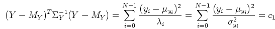
and equation $N(X, M_X, \Sigma_X)=c_0$ becomes $N(Y,M_Y, \Sigma_Y)=c_0$, or

$$(Y-M_Y)^T\Sigma_Y^{-1}(Y-M_Y) =\sum_{i=0}^{N-1} \frac{(y_i-... ...um_{i=0}^{N-1} \frac{(y_i-\mu_{y_i})^2}{\sigma^2_{y_i}} =c_1$$

This equation represents a standard ellipsoid in the N-dimensional space. In other words, KLT $Y=\Phi^T X$ rotates the coordinate system so that the ellipsoid associated with the normal distribution of $X$ becomes a standardized ellipsoid associated with the normal distribution of $Y$, whose axes are parallel to $\phi_i$ ( $i=0, \cdots, N-1$), the axes of the new coordinate system, with the corresponding semi axes equal to $\sqrt{\lambda_i}=\sigma_{y_i}$.

The standardization of the ellipsoid is the essential reason why KLT has the two desirable properties: (a) decorrelation and (b) compaction of energy, as illustrated in the figure: