Next: Comparison with Other Orthogonal
Up: pca
Previous: KLT Completely Decorrelates the
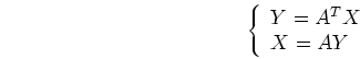
Consider a general orthogonal transform pair defined as
where  and
and  are N by 1 vectors and
  is an arbitrary N by N orthogonal
matrix
is an arbitrary N by N orthogonal
matrix  .
.
We represent by its column vectors
 as
as
or
Now the ith component of can be written as
As we assume the mean vector of is zero  (and obviously we also have
 ), we have
  , and the variance of the ith element in both
and are
, and the variance of the ith element in both
and are
and
where
 and
and
 represent the energy contained in the
ith component of and , respectively. In order words, the trace of
represent the energy contained in the
ith component of and , respectively. In order words, the trace of
 (the sum of all the diagonal elements of the matrix) represents the
expectation of the total amount of energy contained in the signal
(the sum of all the diagonal elements of the matrix) represents the
expectation of the total amount of energy contained in the signal
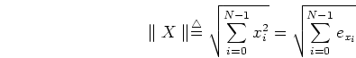
Since an orthogonal transform does not change the length of a vector X,
i.e.,
 ,
where
,
where
the total energy contained in the signal vector is conserved after the
orthogonal transform.
(This conclusion can also be obtained from the fact that orthogonal transforms
do not change the trace of a matrix.)
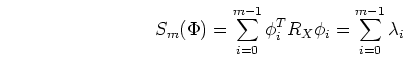
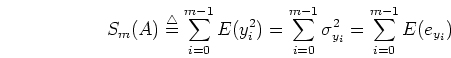
We next define
where  .
.  is a function of the transform matrix and
represents the amount of energy contained in the first
is a function of the transform matrix and
represents the amount of energy contained in the first  components of
  .
Since the total energy is conserved, also represents the percentage
of energy contained in the first components. In the following we will
show that is maximized if and only if the transform is the
KLT:
.
Since the total energy is conserved, also represents the percentage
of energy contained in the first components. In the following we will
show that is maximized if and only if the transform is the
KLT:
i.e., KLT optimally compacts energy into a few components of the signal.
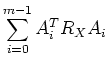
Consider
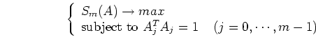
Now we need to find a transform matrix so that
The constraint  is to guarantee that the column vectors in
are normalized. This constrained optimization problem can be solved by Lagrange
multiplier method as shown below.
is to guarantee that the column vectors in
are normalized. This constrained optimization problem can be solved by Lagrange
multiplier method as shown below.
We let
(* the last equal sign is due to explanation in the handout of review of
linear algebra.)
We see that the column vectors of must be the eigenvectors of
 :
:
i.e., the transform matrix must be
Thus we have proved that the optimal transform is indeed KLT, and
where the ith eigenvalue  of is also the average (expectation)
energy contained in the ith component of the signal.
If we choose those
of is also the average (expectation)
energy contained in the ith component of the signal.
If we choose those  that correspond to the largest eigenvalues of
:
that correspond to the largest eigenvalues of
:
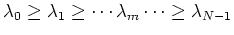 ,
then
,
then  will achieve maximum.
Next: Comparison with Other Orthogonal
Up: pca
Previous: KLT Completely Decorrelates the
Ruye Wang
2004-09-29
![\begin{displaymath}A^{T}=\left[ \begin{array}{c} A_0^{T} . . A_{N-1}^{T} \end{array} \right]
\end{displaymath}](img84.png)

![$\displaystyle \sum_{i=0}^{m-1} E(y_i^2)=
\sum_{i=0}^{m-1} E[A_i^{T}X (A_i^{T}X)^{T}]$](img102.png)
![$\displaystyle \sum_{i=0}^{m-1} E[A_i^{T}X (X^{T}A_i)]
=\sum_{i=0}^{m-1} A_i^{T}E(X X^{T})A_i$](img103.png)
![$\displaystyle \frac{\partial}{\partial A_i}[S_m(A)-\sum_{j=0}^{m-1}
\lambda_j(A_j^{T}A_j-1) ]=0$](img107.png)
![$\displaystyle \frac{\partial}{\partial A_i}[\sum_{j=0}^{m-1}
(A_j^{T}R_XA_j-\lambda_j A_j^{T}A_j+\lambda_j) ]$](img108.png)
![$\displaystyle \frac{\partial}{\partial A_i}
[A_i^{T}R_XA_i-\lambda_i A_i^{T}A_i ]$](img109.png)