PCA

The main idea of principal component analysis (PCA) is to represent the given data points ${\bf x}=[x_1,\cdots,x_d]^T$ in a possibly high d-dimensional space into a space spanned by the eigenvectors of the covariance matrix $\Sigma_x$ of the data points. In the new space the different dimensions (the principal components) of the data points are totally de-correlated and the energy contained in the data, in terms of the sum of the variances in all dimensions, is optimally compacked into a small number of components, so that a large number of components can be discarded without losing much information in the data, i.e., the dimensionality of the space can be much reduced.

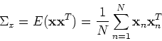
Without loss of generality, we assume the data points have zero mean

$$\mu_x=E({\bf x})=0$$

and the $d\times d$ covariance matrix can be estimated by

$$\Sigma_x=E({\bf x} {\bf x}^T )=\frac{1}{N}\sum_{n=1}^N {\bf x}_n {\bf x}_n^T$$

We then find the eigenvector $\phi_i$ corresponding to the i-th eigenvalue $\lambda_i$ for all $i=1,\cdots,d$:

$$\Sigma_x\phi_i=\lambda_i \phi_i,\;\;\;(i=1,\cdots,d)$$

where the eigenvalues are assumed to be in decreasing order:

$$\lambda_1>\lambda_2>\cdots,\lambda_d$$

A $d\times d$ matrix can be constructed by the eigenvectors as

$$\Phi=[\phi_1,\cdots,\phi_d]$$

and we have

$$\Sigma_x \Phi=\Phi \Lambda,\;\;\;\mbox{or}\;\;\; \Phi^{-1}\Sigma_x \Phi=\Lambda$$

where

$$\Lambda=diag[\lambda_1,\cdots,\lambda_d]$$

Since $\Sigma_x$ is symmectric, its eigenvectors $\phi_i$ are orthogonal to each other $\phi_i^T \phi_j=\delta_{ij}$ and $\Phi^T=\Phi^{-1}$ is orthogonal. Now we have

$$\Phi^T\Sigma_x \Phi=\Lambda$$

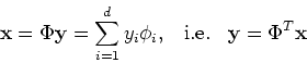
Now all data points ${\bf x}$ can be mapped to a new space spanned by $\phi_1,\cdots,\phi_d$:

$${\bf x}=\Phi {\bf y}=\sum_{i=1}^d y_i \phi_i,\;\;\;\mbox{i.e.}\;\;\; {\bf y}=\Phi^T {\bf x}$$

The i-th component of ${\bf y}=\Phi^T {\bf x}$ is the projection of ${\bf x}$ on the i-th axis $\phi_i$:

$$y_i=(\phi_i,{\bf x})=\phi^T_i {\bf x},\;\;\;\;(i=1,\cdots,d)$$

The covariance matrix in this space is

$$\Sigma_y=E({\bf y}{\bf y}^T)= E(\Phi^T{\bf x}{\bf x}^T\Phi)=\Phi^TE({\bf x}{\bf x}^T)\Phi=\Lambda$$

i.e., all components in the new space are de-correlated:

$$E(y_i y_j)=\sigma^2_{ij}=\delta_{ij}\lambda_i$$

By using only the first few components in ${\bf y}$, we can reduce the dimensionality of the data without losing much of the energy (information) in terms of the sum of the variances in the $d$ components.