convolution

Digital Convolution

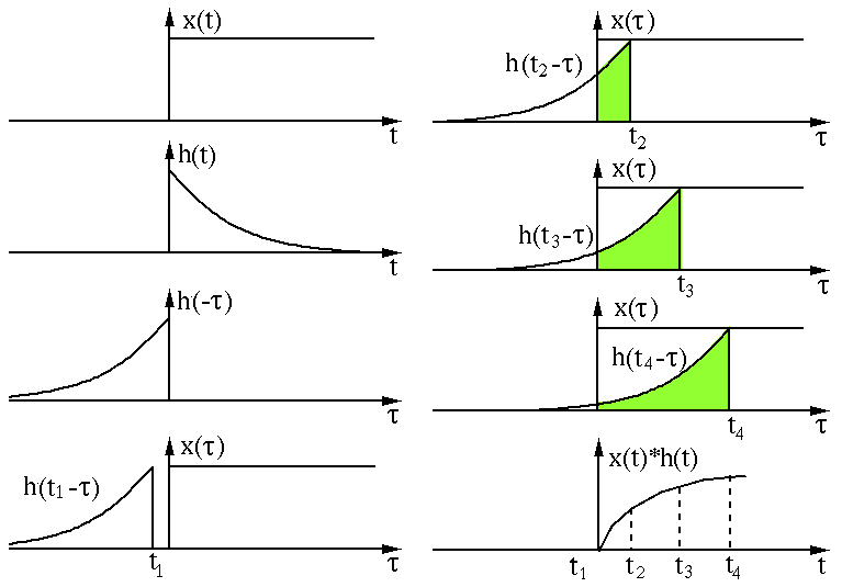
The convolution of two continuous signals $x(t)$ and $h(t)$ is defined as

$\displaystyle y(t)=h(t)*x(t) \stackrel{\triangle}{=} \int_{-\infty}^{\infty} x(\tau) h(t-\tau) d\tau =\int_{-\infty}^{\infty} h(\tau) x(t-\tau) d\tau =x(t)*h(t)$

(1)

i.e., convolution is commutative. Also convolution is associative:

$\displaystyle h*(g*x)=(h*g)*x$

(2)

Typically, $y(t)$

is the output of a system characterized by its impulse response function $h(t)$

with input $x(t)$

. For a finite signal $x(t)=0$

for

and a causal system with $h(t)=0$

for

, we have

$\displaystyle y(t)=h(t)*x(t)=\int_{-\infty}^{\infty} x(\tau) h(t-\tau) d\tau =\int_0^t x(\tau) h(t-\tau) d\tau$

(3)

Convolution in discrete form is

$\displaystyle y[n]=\sum_{m=-\infty}^{\infty} x[n-m] \; h[m] =\sum_{m=-\infty}^{\infty} h[n-m]\;x[m]$

(4)

In image processing, $h[m]$

, the convolution kernel or filter is finite and symmetric:

$\displaystyle h[m] = \left\{ \begin{array}{ll} h[m] & \vert m\vert\le k \\ 0 & \vert m\vert>k \end{array}\right.$

(5)

the convolution becomes

$\displaystyle y[n]=\sum_{m=-k}^{k} x[n-m] \; h[m]$

(6)

If the system in question were a causal system in time domain

$\displaystyle h[n)=h[n]u[n],\;\;\;\;$ i.e. $\displaystyle ,\;\;\;\;h[n]=0\ ;\;\;$ $\displaystyle \mbox{ if $n<0$}$

(7)

the above would become

$\displaystyle y[n]=\sum_{m=0}^{k} x[n-m] \; h[m]$

(8)

However, in image processing, we often consider convolution in spatial domain where causality does not apply.

If $h[m]=h[-m]$ is symmetric (almost always true in image processing), then replacing $m$ by $-m$ we get

$\displaystyle y[n]=\sum_{m=-k}^{k} x[n+m]\;h[-m]=\sum_{m=-k}^{k} x[n+m] \; h[m]$

(9)

We see that now the convolution is the same as the correlation of the two functions.

If the input $x[m]$ is finite (always true in reality), i.e.,

$\displaystyle x[m]=\left\{ \begin{array}{ll} x[m]&0\le m<N\\ 0&otherwise\end{array}\right.$

(10)

its index

in the convolution has to satisfy the following for $x$

to be in the valid non-zero range:

$\displaystyle 0 \le n+m \le N-1$

(11)

or correspondingly, the index $n$

of the output $y[n]$

has to satisfy:

$\displaystyle -m \le n \le N-m-1$

(12)

When the variable index $m$

in the convolution is equal to $k$

, the index of output $y[n]$

reaches its lower bound $n=-k$

; when

, the index of $y[n]$

reaches its upper bound $n=N+k-1$

. In other words, there are $N+2k$

valid (non-zero) elements in the output:

$\displaystyle y[n],\;\;\;\;\;\;(-k \le n \le N+k-1)$

(13)

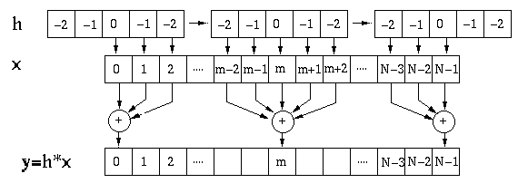
Digital convolution can be best understood graphically (where the index of $y[n]$ is rearranged) as shown below:

We assume the input $x[n]$ has $N$ and the kernel $h$ has $M=2k+1$ (usually an odd number), then the output of the convolution $y=x*h$ has $N-M+1=N-2k$ , as the first component of $y$ corresponds to the $k+1$ component of $x$ (with the $2k+1$ components of $h$ aligned with the first $2k+1$ components of $x$ ). In order for the output $y$ to have the same size as the input $x$ , we can pad the two ends of the input $x$ by $k$ additional components with zeros, zero padding, or repeating values of the end components.

In particular, if the elements of the kernel are all the same (an average operator or a low-pass filter), the we can speed up the convolution process while sliding the kernel over the input signal by taking care of only the two ends of the kernel.

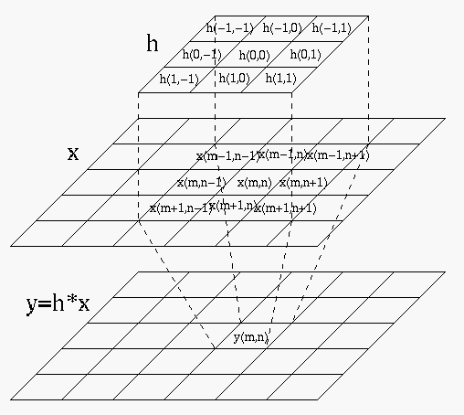
In image processing, all of the discussions above for one-dimensional convolution are generalized into two dimensions, and $h$ is called a convolution kernel, or mask.

$\displaystyle y[m,n]=\sum_{i=-k}^k \sum_{j=-k}^k x[m+i,n+j] h[i,j]$

(14)

About this document ...