The Huffman coding is form of entropy coding which implements the coding idea
discussed above.
If a random number has ![]() possible outcomes (symbols), it is obvious that
these outcomes can be coded by
possible outcomes (symbols), it is obvious that
these outcomes can be coded by ![]() bits. For example, as the pixels in a digital
image can take
bits. For example, as the pixels in a digital
image can take ![]() possible gray values, we need
possible gray values, we need ![]() bits to represent
each pixel and
bits to represent
each pixel and ![]() bits to represent an image of
bits to represent an image of ![]() pixels. By Huffman
coding, however, it is possible to use on average fewer than
pixels. By Huffman
coding, however, it is possible to use on average fewer than ![]() bits to
represent each pixel.
bits to
represent each pixel.
In general, Huffman coding encodes a set of ![]() symbols (e.g.,
symbols (e.g., ![]() gray
levels in a digital image) with binary code of variable length, following this
procedure:
gray
levels in a digital image) with binary code of variable length, following this
procedure:
To illustrate how much compression the Huffman coding can achieve and how the
compression rate is related to the content of the image, consider the following
examples of compressing an image of ![]() gray levels, each with probability
gray levels, each with probability
![]() for a pixel to be at the ith gray level (
for a pixel to be at the ith gray level (![]() ) (the histogram of the
image).
) (the histogram of the
image).
Example 0: ![]() ,
, ![]() , i.e., all pixels take the same value.
The image contains 0 bits uncertainty (no surprise) or information and requires 0
bits to transmit.
, i.e., all pixels take the same value.
The image contains 0 bits uncertainty (no surprise) or information and requires 0
bits to transmit.
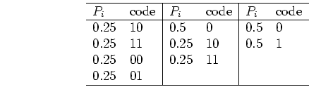
Example 1:
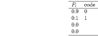
Example 2:
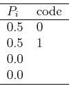
Example 3:
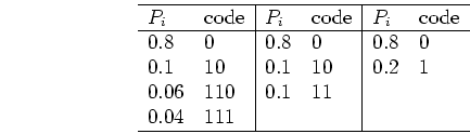
Example 4:
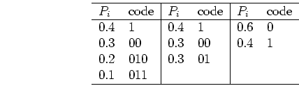
Example 5:
From these examples it can be seen that with variable-length coding the average
number of bits needed to encode a pixel may be reduced from ![]() . The
amount of reduction, or the compression rate, depends on the amount of uncertainty
or information contained in the image. If the image has only a single gray level,
it contains 0 bits information and requires 0 bits to encode; but if the image
has
. The
amount of reduction, or the compression rate, depends on the amount of uncertainty
or information contained in the image. If the image has only a single gray level,
it contains 0 bits information and requires 0 bits to encode; but if the image
has ![]() equally likely gray levels, it contains maximum amount of
equally likely gray levels, it contains maximum amount of ![]() bits
information requiring
bits
information requiring ![]() bits to encode.
bits to encode.