Vector Space and Orthogonal Transform

Definition: A vector space is a set $V$ with two operations of addition and scalar multiplication defined for its members, referred to as vectors.

1. Vector addition maps any two vectors ${\bf x}, {\bf y} \in V$ to another vector ${\bf x}+{\bf y} \in V$ satisfying the following properties:
   • Commutativity: ${\bf x}+{\bf y}={\bf y}+{\bf x}$.
   • Associativity: ${\bf x}+({\bf y}+{\bf z})=({\bf x}+{\bf y})+{\bf z}$.
   • Existence of zero: there is a vector ${\bf0} \in V$ such that: ${\bf0}+{\bf x}={\bf x}+{\bf0}={\bf x}$.
   • Existence of inverse: for any vector ${\bf x}\in V$, there is another vector $-{\bf x}\in V$ such that ${\bf x}+(-{\bf x})={\bf0}$.
2. Scalar multiplication maps a vector ${\bf x}\in V$ and a real or complex scalar $a\in \mathbb{C}$ to another vector $a{\bf x} \in V$ with the following properties:
   • $a({\bf x}+{\bf y})=a{\bf x}+a{\bf y}$.
   • $(a+b){\bf x}=a{\bf x}+b{\bf x}$.
   • $ab{\bf x}=a(b{\bf x})$.
   • $1{\bf x}={\bf x}$.

Definition: An inner product on a vector space $V$ is a function that maps two vectors ${\bf x}, {\bf y} \in V$ to a scalar $\langle {\bf x},{\bf y}\rangle \in \mathbb{C}$ and satisfies the following conditions:

• Positive definiteness:
  
  $$\langle {\bf x},{\bf x}\rangle \;\ge\; 0,\;\;\;\;\;\;\;\; ... ...{\bf x},{\bf x}\rangle =0\;\;\; \mbox{iff}\;\;{\bf x}={\bf0}.$$
  
  

• Conjugate symmetry:
  
  $$\langle {\bf x},{\bf y}\rangle=\overline{\langle {\bf y},{\bf x}\rangle}.$$
  
  
  If the vector space is real, the inner product becomes symmetric:
  
  $$\langle {\bf x},{\bf y}\rangle=\langle {\bf y},{\bf x}\rangle.$$
  
  

• Linearity in the first variable:
  
  $$\langle a{\bf x}+b{\bf y},{\bf z}\rangle=a\langle {\bf x},{\bf z}\rangle+b\langle {\bf y},{\bf z}\rangle,$$
  
  
  where $a,b\in \mathbb{C}$. The linearity does not apply to the second variable:
  

  $$\langle {\bf x}, a{\bf y}+b{\bf z}\rangle=\overline{\langle a{\bf... ...le} =\overline{a\langle {\bf y},{\bf x}\rangle+b\langle {\bf z},{\bf x}\rangle}$$

  $$= \overline{a}\langle {\bf x},{\bf y}\rangle+\overline{b}\langle {\... ... z}\rangle \ne a\langle {\bf x},{\bf y}\rangle+b\langle {\bf x},{\bf z}\rangle,$$

  
  
  unless the coefficients are real $a,b \in \mathbb{R}$. As a special case, when $b=0$, we have
  
  $$\langle a{\bf x},{\bf y}\rangle=a\langle {\bf x},{\bf y}\rang... ... x},a{\bf y}\rangle=\overline{a}\langle {\bf x},{\bf y}\rangle.$$
  
  
  More generally we have
  
  $$\left\langle \sum_n c_n {\bf x}_n,{\bf y}\right\rangle=\sum... ...angle=\sum_n \overline{c}_n \langle {\bf x},{\bf y}_n\rangle.$$
  
  

Definition: A vector space with inner product defined is called an inner product space.

Definition: When the inner product is defined, $\mathbb{C}^N$ is called a unitary space and $\mathbb{R}^N$ is called a Euclidean space.

Examples

• In a vector space (of either finite or infinite dimensionality), the inner product, also called the dot product, of two vectors ${\bf x}=[\cdots,x[n],\cdots]^\textrm{T}$ and ${\bf y}=[\cdots,y[n],\cdots]^\textrm{T}$ is defined as
  
  $$\langle {\bf x}, {\bf y}\rangle={\bf x}^\textrm{T}\overline... ...] \overline{x}[n]} =\overline{\langle{\bf y},{\bf x}\rangle}$$
  
  
  where ${\bf y}^*=\overline{{\bf y}}^\textrm{T}$ is the conjugate transpose of ${\bf y}$. In particular, the sifting property of the delta function
  
  $${\bf d}=[\cdots \cdots,1,\cdots \cdots]^T, \;\;\;\;\mbox{i.... ...]=\left\{ \begin{array}{ll}1&n=0 0&n\ne 0\end{array}\right.$$
  
  
  is an inner product:
  
  $$\langle {\bf x},{\bf d}\rangle=\sum_n x[n] \delta[n] = x[0]$$
  
  

• In a space of 2-D matrices containing $M\times N$ elements, the inner product of two matrices ${\bf x}$ and ${\bf y}$ is defined as
  
  $$\langle {\bf x}, {\bf y}\rangle=\sum_{m=1}^M\sum_{n=1}^N x[m,n]\overline{y}[m,n].$$
  
  
  This inner product is equivalent to previous case if we cascade the column (or row) vectors of ${\bf x}$ and ${\bf y}$ to form two $MN$-D vectors.
• In a function space, the inner product of two function vectors $x(t)$ and $y(t)$ is defined as
  
  $$\langle x(t),y(t)\rangle=\int_a^b x(t)\overline{y(t)} \;dt ... ...verline{x(t)}y(t)} \;dt =\overline{\langle y(t),x(t)\rangle}.$$
  
  
  In particular, the sifting property of the delta function $\delta(t)$ is an inner product:
  
  $$\langle x(t),\delta(t)\rangle=\int_{-\infty}^\infty x(\tau) \delta(\tau) \;d\tau=x(0).$$
  
  

• The inner product of two random variables $x$ and $y$ can be defined as
  
  $$\langle x,y\rangle=E[x\overline{y}].$$
  
  
  If the two random variables have zero means; i.e., $\mu_x=E(x)=0$ and $\mu_x=E(x)=0$, the inner product above is also their covariance:
  
  $$\sigma^2_{xy}=E[(x-\mu_x)\overline{(y-\mu_y)}]= E(x\overline{y})-\mu_x\overline{\mu}_y=E(x\overline{y})=\langle x,y\rangle.$$
  
  

The concept of inner product is of essential importance based on which a whole set of other important concepts can be defined.

Definition: If the inner product of two vectors ${\bf x}$ and ${\bf y}$ is zero, $\langle {\bf x}, {\bf y}\rangle=0$, they are orthogonal (perpendicular) to each other, denoted by ${\bf x}\; \bot\; {\bf y}$.

Definition: The norm (or length) of a vector ${\bf x}\in V$ is defined as

$$\vert\vert{\bf x}\vert\vert=\sqrt{\langle {\bf x},{\bf x}\ran... ... \vert\vert{\bf x}\vert\vert^2=\langle {\bf x},{\bf x}\rangle.$$

The norm $\vert\vert{\bf x}\vert\vert$ is non-negative and it is zero if and only if ${\bf x}={\bf0}$. In particular, if $\vert\vert{\bf x}\vert\vert=1$, then it is said to be normalized and becomes a unit vector. Any vector can be normalized when divided by its own norm: ${\bf x}/\vert\vert{\bf x}\vert\vert$. The vector norm squared $\vert\vert{\bf x}\vert\vert^2=\langle {\bf x},{\bf x}\rangle$ can be considered as the energy of the vector.

Example: In an $N$-D unitary space, the p-norm of a vector ${\bf x}=[x[1],\ldots,x[N]]^\textrm{T} \in \mathbb{C}^N$ is

$$\vert\vert{\bf x}\vert\vert _p=\left[\sum_{n=1}^N \vert x[n]\vert^p\right]^{1/p}.$$

• $p=1$:
  
  $$\vert\vert{\bf x}\vert\vert _1=\sum_{n=1}^N \vert x[n]\vert$$
  
  

• $p=2$
  
  $$\vert\vert{\bf x}\vert\vert=\sqrt{\langle {\bf x},{\bf x}\ran... ...ght]^{1/2} =\left[\sum_{n=1}^N \vert x[n]\vert^2\right]^{1/2}.$$
  
  
  The total energy contained in this vector is its norm squared:
  
  $${\cal E}=\vert\vert{\bf x}\vert\vert^2=\langle {\bf x},{\bf x}\rangle=\sum_{n=1}^N \vert x[n]\vert^2.$$
  
  

• $p=\infty$
  
  $$\vert\vert{\bf x}\vert\vert _\infty=\max(\vert x[1]\vert,\ldots,\vert x[N]\vert).$$
  
  

The concept of $N$-D unitary (or Euclidean) space can be generalized to an infinite-dimensional space, in which case the range of the summation will cover all real integers ${\mathbb Z}$ in the entire real axis $-\infty<n<\infty$. This norm exists only if the summation converges to a finite value; i.e., the vector ${\bf x}$ is an energy signal with finite energy:

$$\sum_{n=-\infty}^\infty \vert x[n]\vert^2 < \infty.$$

All such vectors ${\bf x}$ satisfying the above are square-summable and form the vector space denoted by $l^2({\mathbb Z})$.

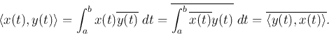
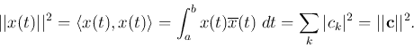
Similarly, in a function space, the norm of a function vector ${\bf x}=x(t)$ is defined as

$$\vert\vert{\bf x}\vert\vert=\left[ \int_a^b x(t)\overline{x(t... ...{1/2} =\left[ \int_a^b \vert x(t)\vert^2\; \;dt \right]^{1/2},$$

where the lower and upper integral limits $a<b$ are two real numbers, which may be extended to all real values $\mathbb{R}$ in the entire real axis $-\infty<t<\infty$. This norm exists only if the integral converges to a finite value; i.e., $x(t)$ is an energy signal containing finite energy:

$$\int_{-\infty}^\infty \vert x(t) \vert^2 \;dt < \infty.$$

All such functions $x(t)$ satisfying the above are square-integrable, and they form a function space denoted by ${\cal L}^2(\mathbb{R})$.

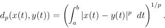
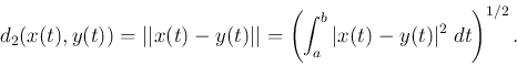
Definition: In a unitary space $\mathbb{C}^N$, the p-norm distance between two vectors ${\bf x}$ and ${\bf y}$ is defined as the p-norm of the difference ${\bf x}-{\bf y}$:

$$d_p({\bf x},{\bf y})=\left( \sum_{n=1}^N \vert x[n]-y[n]\vert^p\right)^{1/p}.$$

• $p=1$
  
  $$d_1({\bf x},{\bf y})&=&\sum_{n=1}^N \vert x[n]-y[n]\vert$$
  
  

• $p=2$
  
  $$d({\bf x},{\bf y})=\vert\vert{\bf x}-{\bf y}\vert\vert=\left(\sum_{n=1}^N \vert x[n]-y[n]\vert^2\right)^{1/2}.$$
  
  
  This is the Euclidean distance between two vectors ${\bf x}$ and ${\bf y}$ defined as the norm of the difference vector ${\bf x}-{\bf y}$.
• $p=\infty$
  
  $$d_\infty({\bf x},{\bf y})&=&\max( \vert x[1]-y[1]\vert,\ldots,\vert x[N]-y[N]\vert).$$
  
  

In a function space, the p-norm distance between two functions $x(t)$ and $y(t)$ is similarly defined as

$$d_p(x(t),y(t))=\left( \int_a^b \vert x(t)-y(t)\vert^p \; \;dt\right)^{1/p}.$$

In particular, when $p=2$, we have

$$d_2(x(t),y(t))=\vert\vert x(t)-y(t)\vert\vert=\left( \int_a^b \vert x(t)-y(t)\vert^2 \;dt\right)^{1/2}.$$

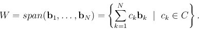
Definition: A vector space V of all linear combinations of a set of vectors ${\bf b}_k\in V,\;(k=1,\ldots,N)$ is called the linear span of the vectors:

$$W=span({\bf b}_1,\ldots,{\bf b}_N) =\left\{ \sum_{k=1}^N c_k {\bf b}_k\;\;\big\vert\;\; c_k \in \mathbb{C} \right\}.$$

Definition: A set of linearly independent vectors that spans a vector space is called a basis of the space. It these vectors are unitary/orthogonal and normalized, they form an orthonormal basis.

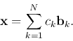
Any vector ${\bf x}\in \mathbb{C}^N$ can be uniquely expressed as a linear combination of some $N$ basis vectors ${\bf b}_k$:

$${\bf x}=\sum_{k=1}^N c_k {\bf b}_k.$$

The concept of a finite $N$-D space spanned by a basis composed of $N$ discrete (countable) linearly independent vectors can be generalized to a vector space V spanned by a basis composed of a family of uncountably infinite vectors ${\bf b}(f)$. Any vector ${\bf x}\in V$ in the space can be expressed as a linear combination, an integral, of these basis vectors:

$${\bf x}=\int_a^b c(f) {\bf b}(f) \;df.$$

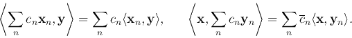
Theorem: Let ${\bf x}$ and ${\bf y}$ be any two vectors in a vector space $V$ spanned by a set of complete orthonormal (orthogonal and normalized) basis vectors $\{ {\bf u}_k \}$ satisfying

$$\langle {\bf u}_k,{\bf u}_l\rangle=\delta[k-l].$$

Then we have

1. Series expansion:
   
   $${\bf x}=\sum_k \langle {\bf x},{\bf u}_k\rangle{\bf u}_k =\s... ...;\;\mbox{where}\;\;\;\; c_k=\langle {\bf x},{\bf u}_k\rangle.$$
   
   
   
   
   $${\bf y}=\sum_k \langle {\bf y},{\bf u}_k\rangle{\bf u}_k =... ...;\mbox{where}\;\;\;\; d_k=\langle {\bf y},{\bf u}_k\rangle.$$
   
   

2. Plancherel theorem:
   
   $$\langle {\bf x},{\bf y}\rangle=\sum_k \langle {\bf x},{\bf ... ...;\;\mbox{where}\;\;\;\; d_k=\langle {\bf y},{\bf u}_k\rangle.$$
   
   

3. Parseval's theorem:
   
   $$\langle {\bf x},{\bf x}\rangle=\vert\vert{\bf x}\vert\vert^2=... ...angle {\bf x},{\bf u}_k\rangle\vert^2=\sum_k \vert c_k\vert^2.$$
   
   

Proof: Taking an inner product with ${\bf u}_l$ on both sides of the first equation we get

$$\langle {\bf x},{\bf u}_l\rangle=\left\langle \sum_k c_k {\bf... ...\langle {\bf u}_k,{\bf u}_l\rangle=\sum_k c_k \delta[k-l]=c_l.$$

Here, ${\bf x}$ is expressed as the vector sum of its projections ${\bf p}_{{\bf u}_k}({\bf x})=\langle {\bf x},{\bf u}_k\rangle {\bf u}_k$ onto each of the unit basis vectors ${\bf u}_k$ and the scalar coefficient $c_k=\langle {\bf x},{\bf u}_k\rangle$ is the norm of the projection.

Example: Space $\mathbb{C}^N$ can be spanned by $N$ orthonormal vectors $\{ {\bf u}_1,\ldots,{\bf u}_N\}$, where the $k$th basis vector is ${\bf u}_k=[u[1,k],\ldots,u[N,k]]^\textrm{T}$, that satisfy:

$$\langle {\bf u}_k,{\bf u}_l\rangle={\bf u}_k^\textrm{T} \over... ...{\bf u}}_l =\sum_{n=1}^N u[n,k]\overline{u}[n,l]=\delta[k-l].$$

Any vector ${\bf x}=[x[1],\ldots,x[N]]^\textrm{T} \in \mathbb{C}^N$ can be expressed as

$${\bf x}=\sum_{k=1}^N c_k {\bf u}_k=[{\bf u}_1,\ldots,{\bf u}_... ...y}{c}c[1] \vdots c[N]\end{array}\right] ={\bf U}{\bf c},$$

where ${\bf c}=[c[1],\ldots,c[N]]^\textrm{T}$ and

$${\bf U}=[{\bf u}_1,\ldots,{\bf u}_N]=\left[ \begin{array}{ccc... ...ts & \vdots \\ u[N,1] & \ldots & u[N,N] \end{array} \right].$$

As the column (and row) vectors in ${\bf U}$ are orthogonal, it is a unitary matrix that satisfies ${\bf U}^{-1}={\bf U}^*$; i.e., ${\bf U}{\bf U}^*={\bf U}^*{\bf U}={\bf I}$ To find the coefficient vector ${\bf c}$, we pre-multiply ${\bf U}^{-1}={\bf U}^*$ on both sides of the previous equation and get:

$${\bf U}^*{\bf x}={\bf U}^{-1}{\bf x}={\bf U}^{-1}{\bf U}{\bf c}={\bf c}.$$

This two equations can be rewritten as a pair of transforms:

$$\left\{ \begin{array}{l} {\bf c}={\bf U}^*{\bf x}={\bf U}^{-1}{\bf x} \\ {\bf x}={\bf U}{\bf c} \end{array} \right..$$

We see that the norm of ${\bf x}$ is conserved (Parseval's identity):

$$\vert\vert{\bf x}\vert\vert^2=\langle {\bf x},{\bf x}\rangle=... ...=\langle {\bf c},{\bf c}\rangle=\vert\vert{\bf c}\vert\vert^2.$$

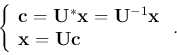
The second equation in the transform pair can also be written in component form as

$$x[n]=\sum_{k=1}^N c_k u[k,n],\;\;\;\;\;\;\;\;\;n=1,\ldots,N.$$

Obviously, the $N$ coefficients $c_k$ ($k=1,\ldots,N$) can be obtained with computational complexity $O(N^2)$.

Example: In ${\cal L}^2$ space composed of all square-integrable functions defined over $a<t<b$, spanned by a set of orthonormal basis functions $u_k(t)$ satisfying:

$$\langle u_k(t),u_l(t)\rangle=\int_a^b u_k(t)\overline{u}_l(t) \;dt=\delta[k-l].$$

Any $x(t)$ in the space can be written as

$$x(t)=\sum_k c_k u_k(t).$$

Taking an inner product with $u_l(t)$ on both sides, we get

$$\langle x(t),u_l(t)\rangle=\sum_k c_k\langle u_k(t), u_l(t)\rangle=\sum_k c_k\delta[k-l]=c_l;$$

i.e.,

$$c_k=\langle x(t), u_k(t)\rangle=\int_a^b x(t)\overline{u}_k(t) \;dt.$$

which is the projection of $x(t)$ onto the unit basis function $\phi_k(t)$. Again we can easily get:

$$\vert\vert x(t)\vert\vert^2=\langle x(t),x(t)\rangle=\int_a^b... ...t) \;dt=\sum_k \vert c_k\vert^2=\vert\vert{\bf c}\vert\vert^2.$$

The Fourier transforms

Consider the following four Fourier bases that span four different types of vector spaces for signals that are either continuous or discrete, of finite or infinite duration.

• ${\bf u}_k=[e^{j2\pi k0/N},\ldots,e^{j2\pi k(N-1)/N}]^\textrm{T}/\sqrt{N}$ ( $k=0,\ldots,N-1$) form a set of $N$ orthonormal basis vectors that span $\mathbb{C}^N$:
  
  $$\langle {\bf u}_k,{\bf u}_l\rangle=\frac{1}{N}\sum_{n=0}^{N-1} e^{j2\pi (k-l)n/N}=\delta[k-l].$$
  
  
  Any vector ${\bf x}=[x[0],\ldots,x[N-1] ]^\textrm{T}$ in $\mathbb{C}^N$ can be expressed as
  
  $${\bf x}=\sum_{k=0}^{N-1} X[k]{\bf u}_k =\sum_{k=0}^{N-1} \langle {\bf x},{\bf u}_k\rangle {\bf u}_k,$$
  
  
  or in component form:
  
  $$x[n]=\frac{1}{\sqrt{N}}\sum_{k=0}^{N-1} X[k] e^{j2\pi kn/N}\;\;\;\;\;\;\;0\le n\le N-1,$$
  
  
  where the coefficient $X[k]$ is the projection of ${\bf x}$ onto ${\bf u}_k$:
  
  $$X[k]=\langle {\bf x},{\bf u}_k\rangle=\sum_{n=0}^{N-1} x[n]\o... ...k] =\frac{1}{\sqrt{N}} \sum_{n=0}^{N-1} x[n] e^{-j2\pi nk/N}.$$
  
  

• ${\bf u}(f)=[\ldots,e^{j2\pi mf/F},\ldots]^\textrm{T}/\sqrt{F}$ ($0<f<F$) form a set of uncountably infinite orthonormal basis vectors (of infinite dimensions) that spans $l^2$ space of all square-summable vectors of infinite dimensions:
  
  $$\langle {\bf u}_f,{\bf u}_{f'}\rangle=\frac{1}{F}\sum_{m=-\infty}^\infty e^{j2\pi (f-f')m/F}=\delta(f-f').$$
  
  

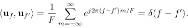
  Any vector ${\bf x}=[\ldots,x[n],\ldots]^\textrm{T}$ in this space can be expressed as
  

  $${\bf x}=\int_{-\infty}^\infty X(f){\bf u}(f) \;df =\int_{-\infty}^\infty \langle {\bf x},{\bf u}(f)\rangle {\bf u}(f) \;df,$$
  
  
  or in component form:
  
  $$x[n]=\frac{1}{\sqrt{F}}\int_{-\infty}^\infty X(f)e^{j2\pi f n/F} \;df,\;\;\;\;\; -\infty<n<\infty,$$
  
  
  where the coefficient function $X(f)$ is the projection of ${\bf x}$ onto ${\bf u}(f)$:
  
  $$X(f)=\langle {\bf x},{\bf u}(f)\rangle=\frac{1}{\sqrt{F}}\sum_{n=-\infty}^\infty x[n]e^{-j2\pi f n/F}.$$
  
  

• $u_k(t)=e^{j2\pi kt/T}/\sqrt{T}$ ( $-\infty<k<\infty$) form a set of infinite orthonormal basis functions that spans the space of all square-integrable functions defined over $0<t<T$:
  
  $$\langle u_k(t),u_l(t)\rangle=\frac{1}{T}\int_0^\textrm{T} e^{j2\pi (k-l)t/T} \;dt=\delta[k-l].$$
  
  
  Any function $x_T(t)$ in this space can be expressed as
  
  $$x_T(t)=\sum_{k=-\infty}^\infty X[k]u_k(t) =\frac{1}{\sqrt{T}}\sum_{k=-\infty}^\infty X[k]e^{j2\pi kt/T},$$
  
  
  where the coefficient $X[k]$ is the projection of $x(t)$ onto the $k$th basis function $u_k(t)$:
  
  $$X[k]=\langle x(t),u_k(t)\rangle=\int_{-\infty}^\infty x(t)\... ...1}{\sqrt{T}}\int_{-\infty}^\infty x(t)e^{-j2\pi kt/T} \;dt.$$
  
  

• $u_f(t)=e^{j2\pi ft}$ ( $-\infty<f<\infty$) is a set of uncountably infinite orthonormal basis functions that spans ${\cal L}^2$ space of all square-integrable functions defined over $-\infty<t<\infty$.
  
  $$\langle u_f(t),u_{f'}(t)\rangle=\int_{-\infty}^\infty e^{j2\pi (f-f')t} \;dt=\delta(f-f').$$
  
  
  Any function $x(t)$ in this space can be expressed as
  
  $$x(t)=\int_{-\infty}^\infty X(f)u_f(t) \;df =\int_{-\infty}^\infty X(f)e^{j2\pi ft} \;df,$$
  
  
  where the coefficient function is the projection of $x(t)$ onto $u_f(t)$:
  
  $$X(f)=\langle x(t),u_f(t)\rangle=\int_{-\infty}^\infty x(t)\... ...}_f(t) \;df =\int_{-\infty}^\infty x(t)e^{-j2\pi ft} \;dt.$$
  
  

Definition: A linear transformation $U: V\rightarrow W$ is a unitary transformation if it conserves inner products:

$$\langle {\bf x},{\bf y}\rangle=\langle U{\bf x},U{\bf y}\rangle.$$

In particular, if the vectors are real with symmetric inner product $\langle {\bf x},{\bf y}\rangle=\langle {\bf y},{\bf x}\rangle$, then $U$ is an orthogonal transformation.

A unitary transformation also conserves any measurement based on the inner product, such as the norm of a vector, the distance and angle between two vectors, and the projection of one vector on another. Also, if in particular ${\bf x}={\bf y}$, we have

$$\langle {\bf x},{\bf x}\rangle=\vert\vert{\bm f}\vert\vert^... ...gle U{\bf x},U{\bf x}\rangle=\vert\vert U{\bf x}\vert\vert^2;$$

i.e., the unitary transformation conserves the vector norm (length). This is Parseval's identity for a generic unitary transformation $U{\bm x}$. Owing to this property, a unitary operation $R: V \rightarrow V$ can be intuitively interpreted as a rotation in space $V$.

Definition A matrix ${\bf U}$ is unitary if it conserves inner products:

$$\langle {\bf U}{\bf x},{\bf U}{\bf y}\rangle=\langle {\bf x},{\bf y}\rangle.$$

Theorem: A matrix ${\bf U}$ is unitary if and only if ${\bf U}^*{\bf U}={\bf I}$; i.e., the following two statements are equivalent:

$$(a) \langle {\bf U}{\bf x},{\bf U}{\bf y}\rangle=\langle {\bf x},{\bf y}\rangle$$

$$(b) {\bf U}^*{\bf U}={\bf U}{\bf U}^*={\bf I};\;\;\;\;\; \mbox{i.e.,}\;\;\;\;\;\;{\bf U}^{-1}={\bf U}^*.$$

When ${\bf U}=\overline{{\bf U}}$ is real, it is an orthogonal matrix.

A unitary matrix ${\bf U}$ has the following properties:

• Unitary transformation ${\bf U}{\bf x}$ conserves the vector norm; i.e., $\vert\vert{\bf U}{\bf x}\vert\vert=\vert\vert{\bf x}\vert\vert$ for any ${\bf x}\in \mathbb{C}^N$.
• All eigenvalues $\{\lambda_1,\ldots,\lambda_N\}$ of ${\bf U}$ have an absolute value of 1: $\vert\lambda_k\vert=1$; i.e., they lie on the unit circle in the complex plain.
• The determinant of ${\bf U}$ has an absolute value of 1: $\vert det({\bf U})\vert=1$. This can be easily seen as $det({\bf U})=\prod_{k=1}^N \lambda_k$.
• All column (or row) vectors of ${\bf U}=[{\bf u}_1,\ldots,{\bf u}_N]$ are orthonormal:
  
  $$\langle {\bf u}_k,{\bf u}_l\rangle=\delta[k-l].$$
  
  

The last property indicates that the column (row) vectors $\{ {\bf u}_k \}$ form an orthogonal basis that spans $\mathbb{C}^N$.

The identity matrix ${\bf I}=[{\bf e}_1,\ldots,{\bf e}_N]$ is a special orthogonal matrix as its columns (or rows) are orthonormal:

$$\langle {\bf e}_k,{\bf e}_l\rangle=\delta[k-l].$$

where the kth vector ${\bf e}_k=[0,\cdots,0,1,0,\cdots,0]^T$ has all zero elements except the kth one being 1. These vectors form the standard basis of $\mathbb{C}^N$. Any vector ${\bf x}=[x[1],\ldots,x[N]]^\textrm{T} \in \mathbb{C}^N$ can be represented by the standard basis as

$${\bf x}=\left[\begin{array}{c}x[1] \vdots x[N]\end{array}... ...ray}{c}x[1] \vdots x[N]\end{array}\right] ={\bf I}{\bf x}$$

The vector can also be represented by any other orthonormal basis ${\bf U}=[{\bf u}_1,\ldots,{\bf u}_N]$ as

$${\bf x}={\bf I}{\bf x}={\bf U} {\bf U}^*{\bf x}={\bf U} {\bf ... ...\vdots c[N]\end{array}\right] =\sum_{k=1}^N c[k] {\bf u}_k,$$

where we have defined

$${\bf c}=\left[\begin{array}{c}c[1] \vdots c[N]\end{array}... ...;\; c[k]={\bf u}_k^*{\bf x}=\langle {\bf x},{\bf u}_k\rangle.$$

Combining the two equations we get

$$\left\{ \begin{array}{l} {\bf c}={\bf U}^*{\bf x},\\ {\bf x}={\bf U}{\bf c}. \end{array}\right.$$

This is the generalized Fourier transform, by which a vector ${\bf x}$ is rotated to become another vector ${\bf c}$.

This result can be extended to the continuous transformation for signal vectors in the form of continuous functions. In general, corresponding to any given unitary transformation $U$, a signal vector ${\bf x}\in V$ can be alternatively represented by a coefficient vector ${\bf c}=U^*{\bf x}$ (where ${\bf c}$ can be either a set of discrete coefficients $c_k$ or a continuous function $c(f)$). The original signal vector ${\bf x}$ can always be reconstructed from ${\bf c}$ by applying $U$ on both sides of ${\bf c}=U^*{\bf x}$ to get $U{\bf c} =UU^*{\bf x}=I{\bf x}={\bf x}$; i.e., we get a unitary transform pair in the most general form:

$$\left\{ \begin{array}{l} {\bf c}=U^*{\bf x},\\ {\bf x}=U{\bf c}. \end{array}\right.$$

The first equation is the forward transform that maps the signal vector ${\bf x}$ to a coefficient vector ${\bf c}$, while the second equation is the inverse transform by which the signal is reconstructed.